Draw a schematic representation of a process

A generic method for drawing a schematic representation of processes-type classes.

Usage

draw(object, ...)

draw.technology(
  object,
  ...,
  vintage = NULL,
  cluster = NULL,
  ghost = ghost_options(),
  cluster_style = c("rail", "deck", "none"),
  box_width = 0.4,
  max_facets = 24L
)

# S4 method for class 'technology'
draw(object, ...)

# S4 method for class 'storage'
draw(object, ...)

# S4 method for class 'supply'
draw(object, ...)

# S4 method for class 'demand'
draw(object, ...)

# S4 method for class 'export'
draw(object, ...)

# S4 method for class 'import'
draw(object, ...)

# S4 method for class 'trade'
draw(object, ...)

Arguments

object: The object to draw: technology, storage, trade, demand, supply, export, or import.
...: Additional arguments passed to the specific method.
vintage: which vintage to draw in full for a vintaged technology: a level name, an index, NULL (the default, the newest one), or "all" to lay every vintage out side by side at full detail. Other vintages are drawn as faded ghosts behind the selected one – earlier to the left, later to the right.
cluster: which cluster to draw, in the same forms as vintage. The default NULL takes the FIRST declared cluster, declarations ranking clusters best-resource-first. Clusters are not fanned out like vintages: they coexist rather than succeed one another, and a technology can carry dozens, so the axis is drawn as an index (see cluster_style).
ghost: geometry of the ghost stack: a ghost_options() object, or a named list of overrides.
cluster_style: how to show the cluster axis: "rail" (the default) a strip of ticks with the selection filled, "deck" slivers at the box edge suggesting a stack of cards, or "none".
max_facets: refuse to lay out more than this many panels for vintage = "all" / cluster = "all". A full 11 x 4 grid is unreadable, and silently drawing it is worse than saying so.
region: A node to draw the trade process for. node is an alias for region. Default is the first node in the trade object.

Value

displays a schematic representation of the process, returns NULL.

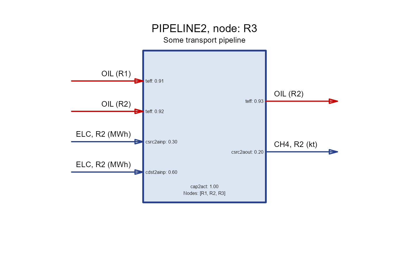
A figure with a schematic representation of the export process.

A figure with a schematic representation of the import process.

Examples

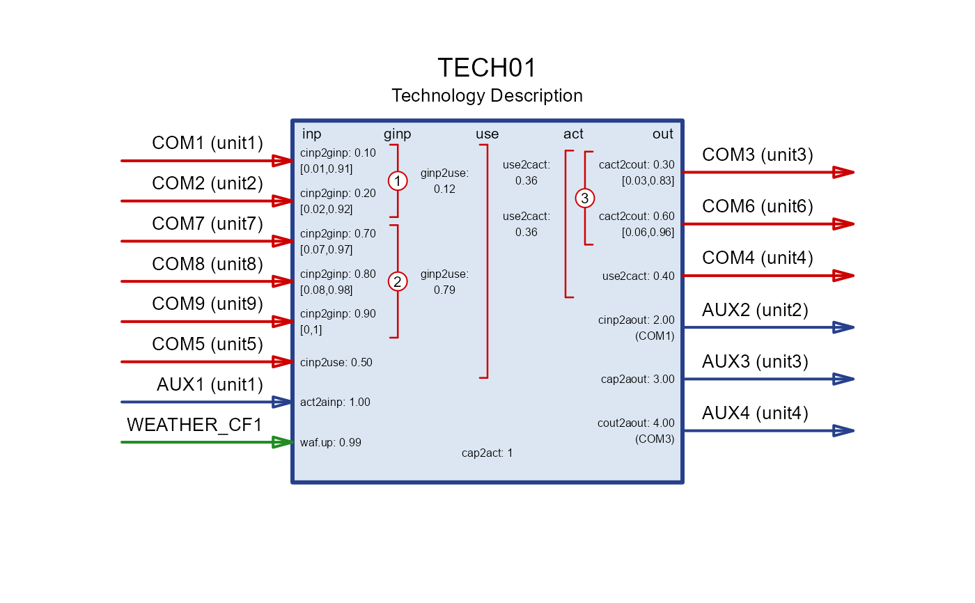
TECH01 <- newTechnology(
  "TECH01",
  desc = "Technology Description",
  input = data.frame(
    comm = c("COM1", "COM2", "COM5", "COM7", "COM8", "COM9"),
    group = c("1", "1", NA, "2", "2", "2"),
    unit = c("unit1", "unit2", "unit5", "unit7", "unit8", "unit9")
  ),
  output = data.frame(
    comm = c("COM3", "COM4", "COM6"),
    group = c("3", NA, "3"),
    unit = c("unit3", "unit4", "unit6")
  ),
  group = data.frame(
    group = c("1", "2", "3"),
    desc = c("Group1", "Group2", "Group3"),
    unit = "unit"
  ),
  aux = data.frame(
    acomm = c("AUX1", "AUX2", "AUX3", "AUX4"),
    unit = c("unit1", "unit2", "unit3", "unit4")
  ),
  region = c("R1", "R2", "R3"),
  geff = data.frame(
    group = c("1", "2"),
    ginp2use = c(0.12, 0.789)
  ),
  ceff = data.frame(
    comm = c("COM1", "COM2", "COM5", "COM7", "COM8", "COM9", "COM3", "COM4", "COM6"),
    cinp2ginp = c(.1, .2, NA, .7, .8, .9, rep(NA, 3)),
    cinp2use = c(NA, NA, .5, NA, NA, NA, rep(NA, 3)),
    use2cact = c(rep(NA, 6), .36, .4, .36),
    cact2cout = c(rep(NA, 6), .3, NA, .6),
    share.lo = c(.01, .02, NA, .07, .08, .0, .03, NA, .06),
    share.up = c(.91, .92, NA, .97, .98, 1, .83, NA, .96)
  ),
  aeff = data.frame(
    acomm = c("AUX1", "AUX2", "AUX3", "AUX4"),
    comm = c(NA, "COM1", NA, "COM3"),
    act2ainp = c(1, NA, NA, NA),
    cinp2aout = c(NA, 2, NA, NA),
    cap2aout = c(NA, NA, 3, NA),
    cout2aout = c(NA, NA, NA, 4)
  ),
  weather = data.frame(
    weather = "WEATHER_CF1",
    waf.up = .99
  )
)
draw(TECH01)

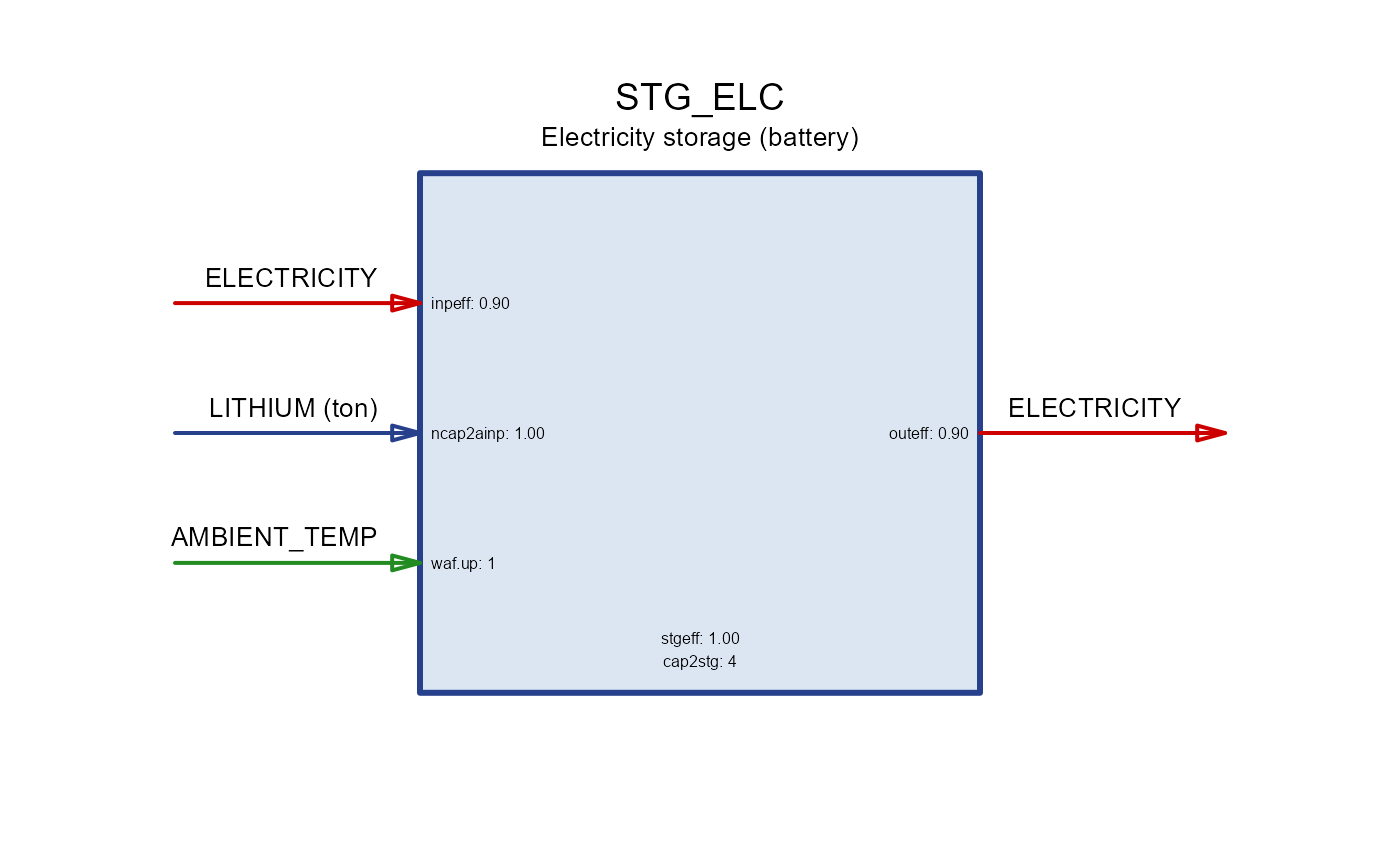
STG_ELC <- newStorage(
  name = "STG_ELC", # used in sets
  desc = "Electricity storage (battery)", # for own reference
  commodity = "ELECTRICITY", # must match the commodity name in the model
  aux = data.frame(
    acomm = "LITHIUM", # auxiliary commodity for battery production
    unit = "ton" # unit of the auxiliary commodity
  ),
  start = data.frame(
    start = 2020 # the first year of the process is available for installation
  ),
  end = data.frame(
    end = 2030 # last year of the process is available for installation
  ),
  olife = data.frame(
    olife = 20 # operational life of the storage in years
  ),
  seff = data.frame(
    stgeff = 0.999, # storage efficiency
    inpeff = 0.9, # charging efficiency
    outeff = 0.9 # discharging efficiency
  ),
  aeff = data.frame(
    acomm = "LITHIUM", # track lithium use for battery production
    ncap2ainp = convert(4 * 250, "Wh/kg", "GWh/kt") # lithium per energy capacity
  ),
  af = data.frame(
    # af.lo = 0., # lower bound for the capacity factor
    af.up = 1. # upper bound for the capacity factor
  ),
  fixom = data.frame(
    # region = "R1",
    # year = 2020,
    fixom = 0.9 # fixed operation and maintenance cost
  ),
  duration = 4, # four-hours of storage
  invcost = data.frame(
    region = c("R1", NA), # region R1 and all other regions
    invcost = c(1e3, 1.1e3) # investment cost in MUSD/GWh of 4-hour storage
  ),
  fullYear = TRUE, # full year storage cycle
  weather = data.frame(
    weather = "AMBIENT_TEMP", # weather factor for capacity factor
    waf.up = 1 # affects upper boundary of capacity factor
    # waf.lo = 0.9 # affects lower boundary of capacity factor
  )
  # region = c("R1", "R2", "R3"),
)
draw(STG_ELC)


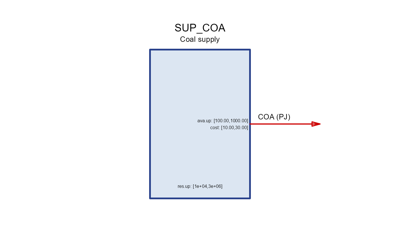
SUP_COA <- newSupply(
  name = "SUP_COA",
  desc = "Coal supply",
  commodity = "COA",
  unit = "PJ",
  reserve = data.frame(
    region = c("R1", "R2", "R3"),
    res.up = c(2e5, 1e4, 3e6) # total reserves/deposits
  ),
  supply = data.frame(
    region = c("R1", "R2", "R3"),
    year = NA_integer_,
    timeslice = "ANNUAL",
    ava.up = c(1e3, 1e2, 2e2), # annual availability
    cost = c(10, 20, 30) # cost of the resource (currency per unit)
  ),
  region = c("R1", "R2", "R3")
)
draw(SUP_COA)

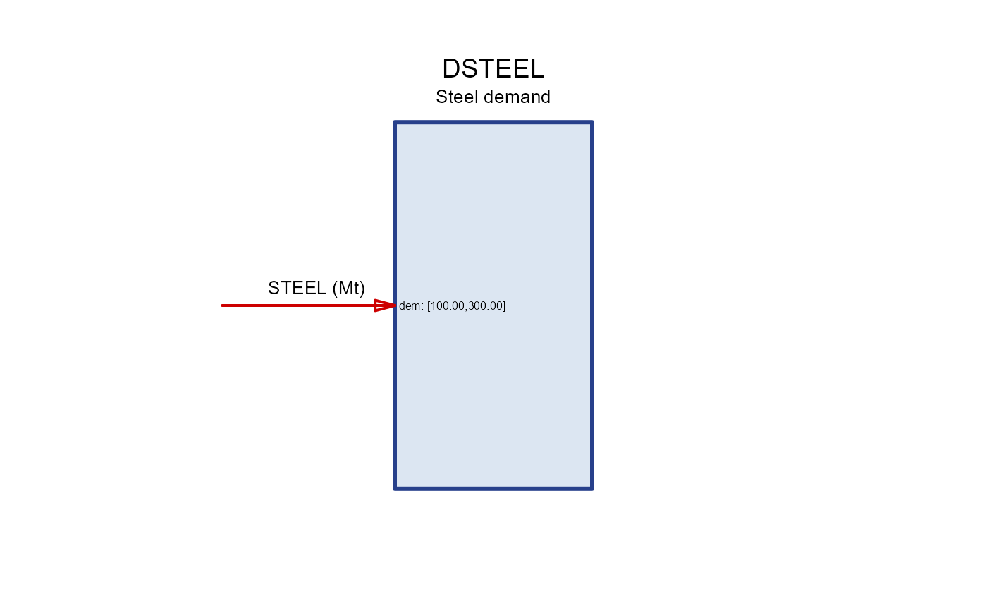
DSTEEL <- newDemand(
  name = "DSTEEL",
  desc = "Steel demand",
  commodity = "STEEL",
  unit = "Mt",
  demand = data.frame(
    region = "UTOPIA", # NA for every region
    year = c(2020, 2030, 2050),
    timeslice = "ANNUAL",
    demand = c(100, 200, 300)
  ),
  region = "UTOPIA", # optional, to narrow the specification of the demand
)
draw(DSTEEL)

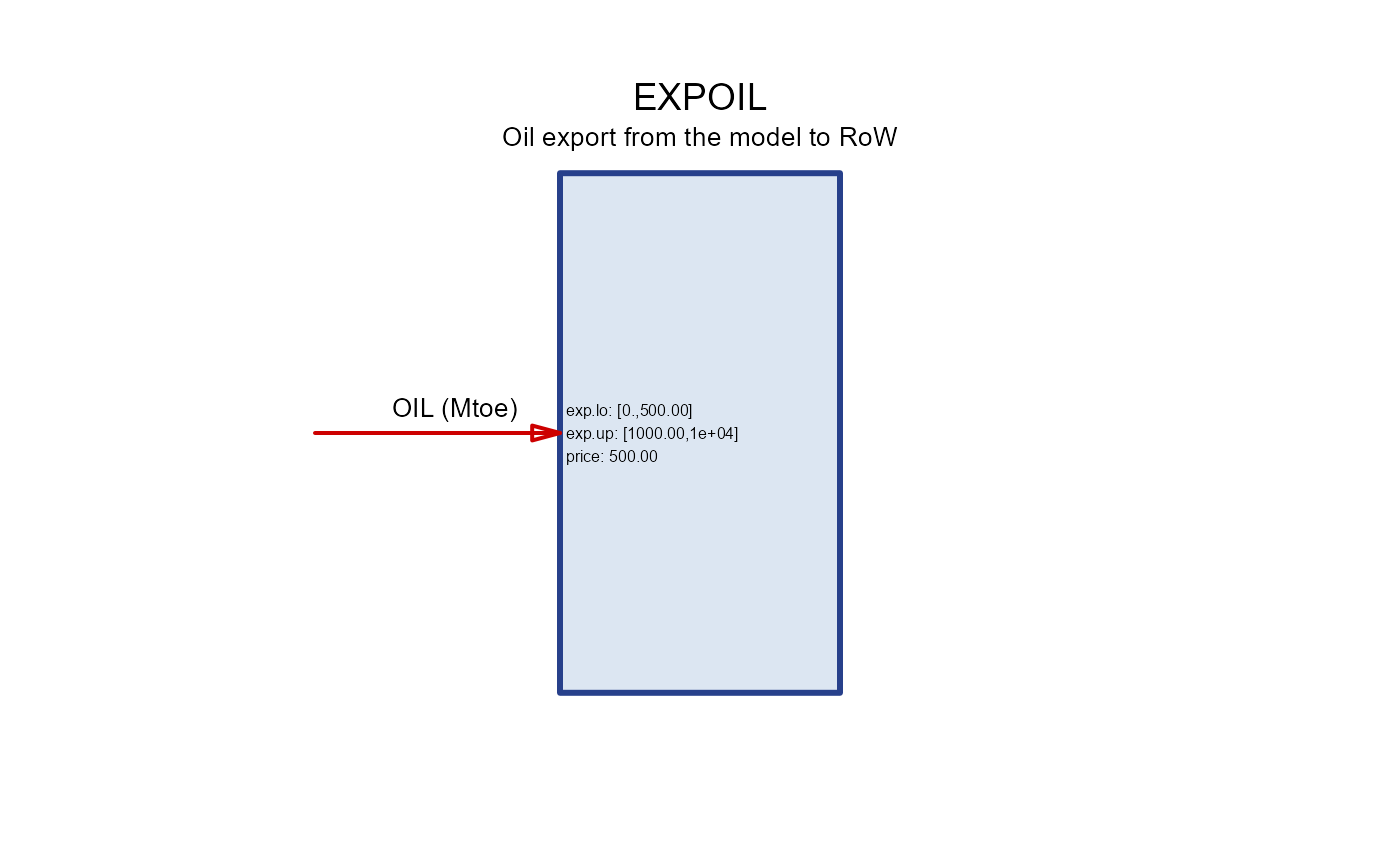
EXPOIL <- newExport(
  name = "EXPOIL", # used in sets
  desc = "Oil export from the model to RoW", # for own reference
  commodity = "OIL", # must match the commodity name in the model
  unit = "Mtoe", # for own reference
  exp = data.frame(
    region = rep(c("R1", "R2"), each = 2), # export region(s)
    year = rep(c(2020, 2050)), # export years
    price = 500, # export price in MUSD/Mtoe (USD/t),
    exp.up = rep(c(1e3, 1e4), each = 2), # upper bound for export in each year
    exp.lo = rep(c(5e2, 0), each = 2) # lower bound for export in each year
  )
)
draw(EXPOIL)

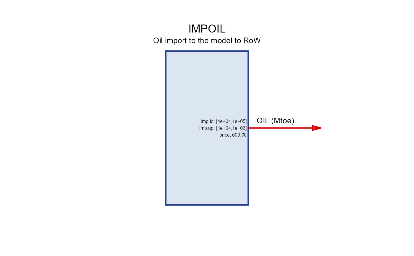
IMPOIL <- newImport(
  name = "IMPOIL", # used in sets
  desc = "Oil import to the model to RoW", # for own reference
  commodity = "OIL", # must match the commodity name in the model
  unit = "Mtoe", # for own reference
  imp = data.frame(
    region = rep(c("R1", "R2"), each = 2), # import region(s)
    year = rep(c(2020, 2050)), # import years
    price = 600, # import price in MUSD/Mtoe (USD/t),
    imp.up = rep(c(1e4, 1e6), each = 2), # upper bound for import in each year
    imp.lo = rep(c(1e4, 1e5), each = 2) # lower bound for import in each year
  )
)
draw(IMPOIL)

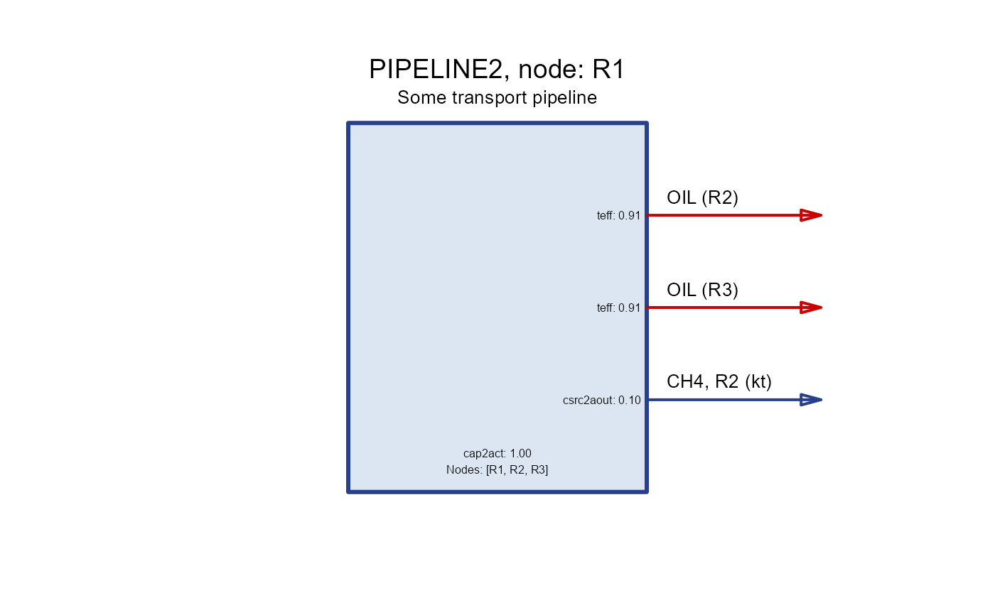
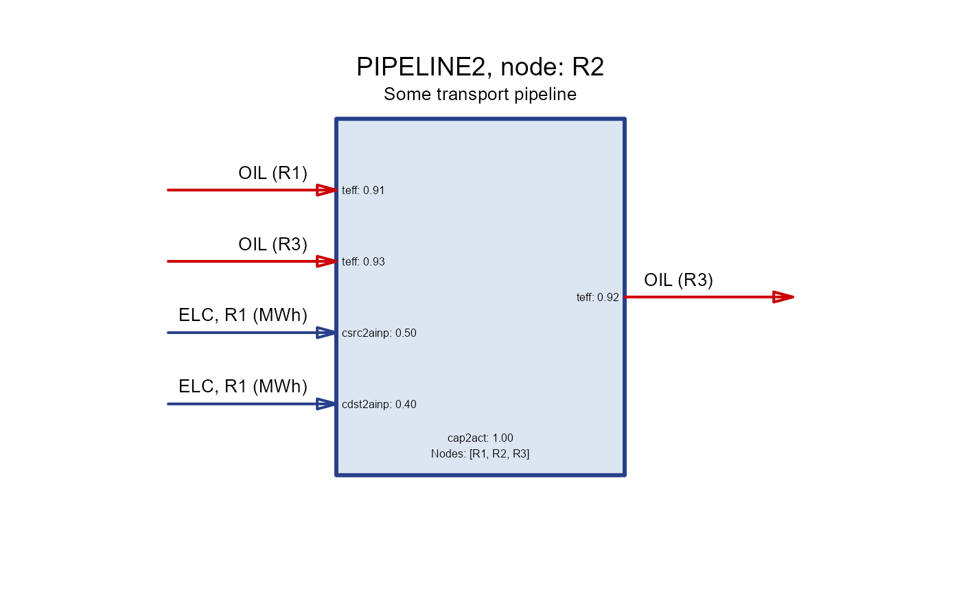
PIPELINE2 <- newTrade(
  name = "PIPELINE2",
  desc = "Some transport pipeline",
  commodity = "OIL",
  routes = data.frame(
    src = c("R1", "R1", "R2", "R3"),
    dst = c("R2", "R3", "R3", "R2")
  ),
  trade = data.frame(
    src = c("R1", "R1", "R2", "R3"),
    dst = c("R2", "R3", "R3", "R2"),
    teff = c(0.912, 0.913, 0.923, 0.932)
  ),
  aux = data.frame(
    acomm = c("ELC", "CH4"),
    unit = c("MWh", "kt")
  ),
  aeff = data.frame(
    acomm = c("ELC", "CH4", "ELC", "CH4"),
    src = c("R1", "R1", "R2", "R3"),
    dst = c("R2", "R2", "R3", "R2"),
    csrc2ainp = c(.5, NA, .3, NA),
    cdst2ainp = c(.4, NA, .6, NA),
    csrc2aout = c(NA, .1, NA, .2)
  ),
  olife = list(olife = 60)
)
draw(PIPELINE2, node = "R1")

draw(PIPELINE2, node = "R2")

draw(PIPELINE2, node = "R3")

Draw a schematic representation of a process

Usage

Arguments

Value

See also

Examples