Processes: technology, storage, trade, supply, demand, import, export

Processes are the model elements that move and convert commodities. energyRt has seven of them, and every one has a draw() method that renders a schematic of its inputs, outputs, auxiliary commodities and key coefficients.

Process	Role	Main commodity flow
`supply`	domestic source of a commodity	→ out
`demand`	final consumption (a sink)	in →
`import`	purchase from the rest of the world	→ out
`export`	sale to the rest of the world	in →
`trade`	move a commodity between regions	in ↔︎ out (per region)
`storage`	shift a commodity across time	in → $store$ → out
`technology`	convert input commodities into outputs	in → use → activity → out

library(energyRt)

The process family

A one-line example and its diagram for each of the simpler processes.

supply

A source of a commodity, with an availability bound and a cost (see the autoplot article for the by-year view of the same data).

SUP_COA <- newSupply(
  name = "SUP_COA", desc = "Coal supply", commodity = "COA", unit = "PJ",
  reserve = data.frame(region = "R1", res.up = 2e5),
  availability = data.frame(region = "R1", year = NA_integer_, slice = "ANNUAL",
                            ava.up = 1e3, cost = 10))
draw(SUP_COA)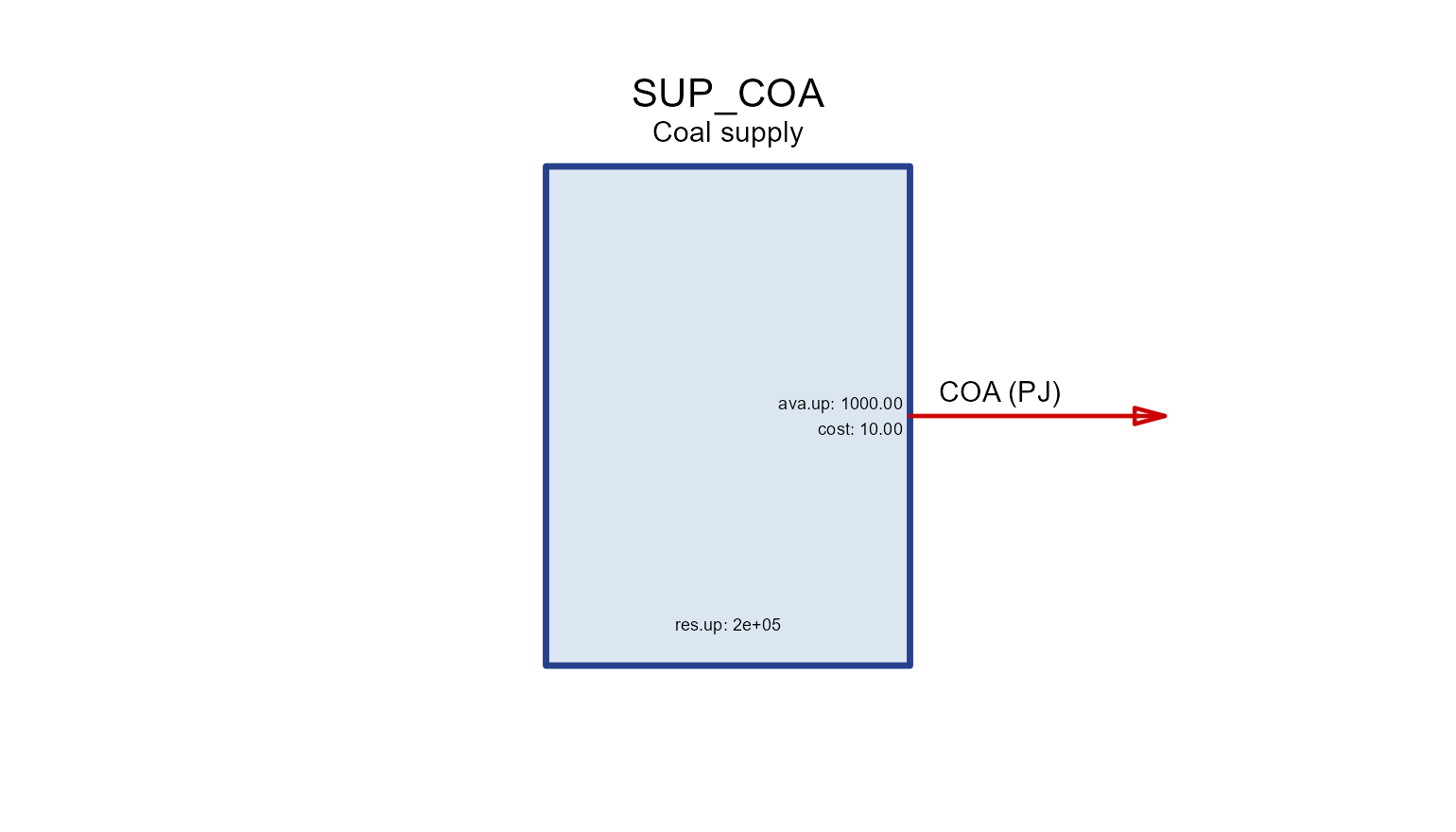

demand

A commodity sink; dem is the demanded quantity over years/slices.

DEM_ELC <- newDemand(
  name = "DEM_ELC", desc = "Electricity demand", commodity = "ELC", unit = "GWh",
  dem = data.frame(region = "R1", year = c(2020, 2050), slice = "ANNUAL",
                   dem = c(100, 300)))
draw(DEM_ELC)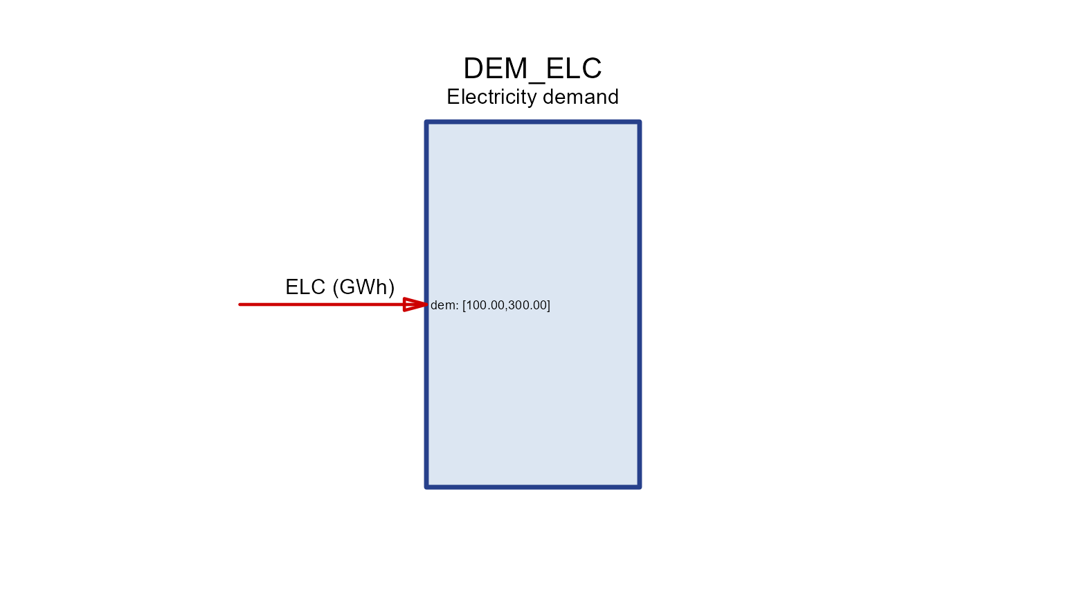

import / export

Trade with the “rest of the world” at a price, bounded by imp.* / exp.*.

IMP_GAS <- newImport(
  name = "IMP_GAS", desc = "Gas import", commodity = "GAS", unit = "PJ",
  imp = data.frame(region = "R1", year = c(2020, 2050), price = 6, imp.up = 500))
draw(IMP_GAS)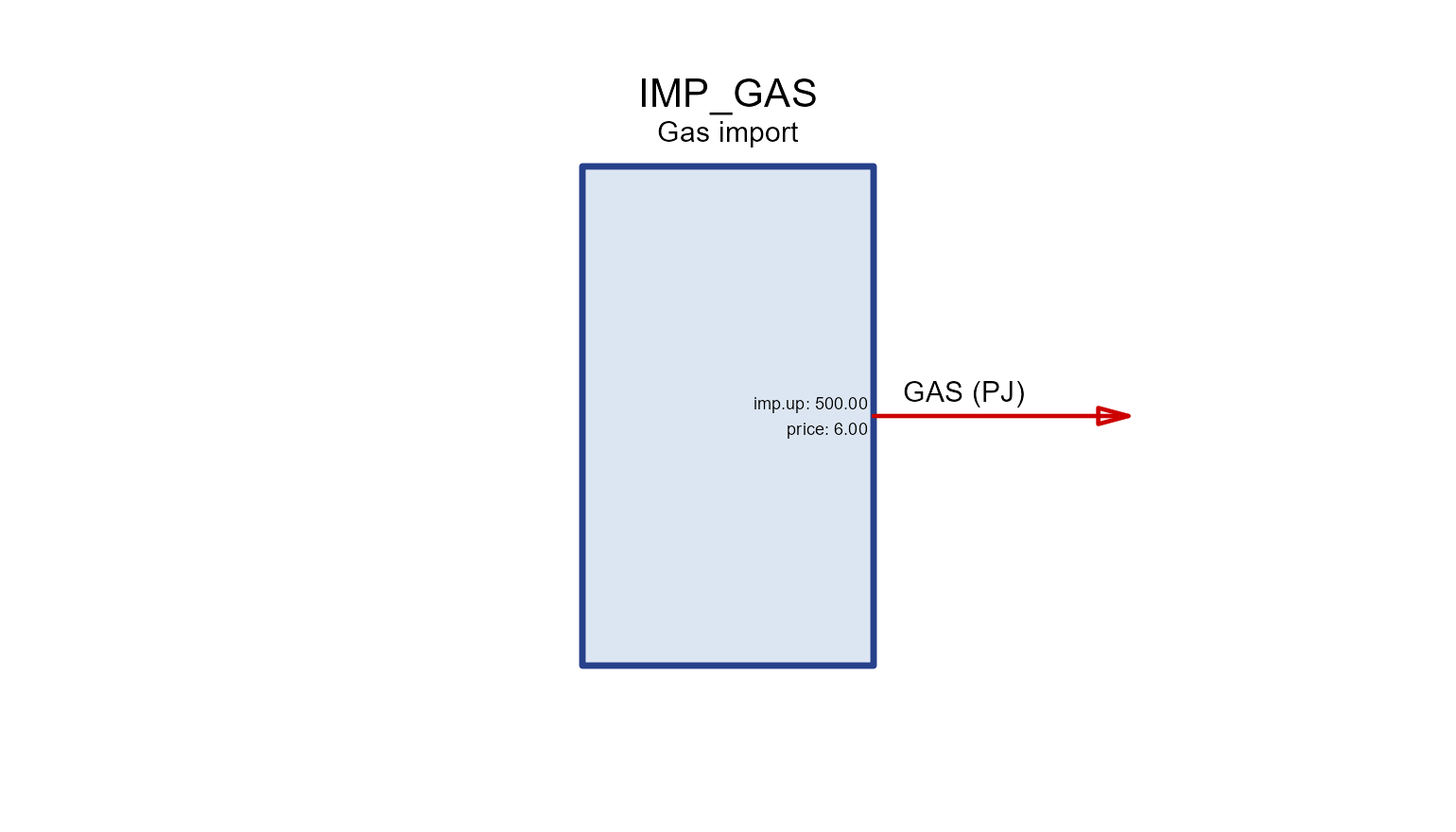


EXP_OIL <- newExport(
  name = "EXP_OIL", desc = "Oil export", commodity = "OIL", unit = "Mt",
  exp = data.frame(region = "R1", year = c(2020, 2050), price = 500, exp.up = 100))
draw(EXP_OIL)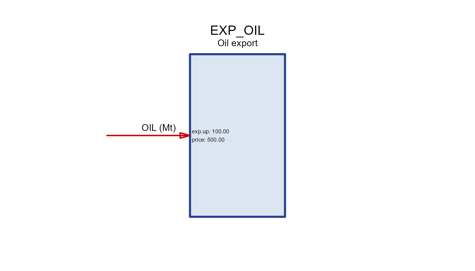

trade

Moves a commodity along routes (src → dst) between regions with a transport efficiency teff. draw() shows the flows for one node at a time.

PIPE <- newTrade(
  name = "PIPE", desc = "Gas pipeline", commodity = "GAS",
  routes = data.frame(src = c("R1", "R2"), dst = c("R2", "R3")),
  trade  = data.frame(src = c("R1", "R2"), dst = c("R2", "R3"), teff = c(0.97, 0.96)))
draw(PIPE, node = "R2")   # imports from R1, exports to R3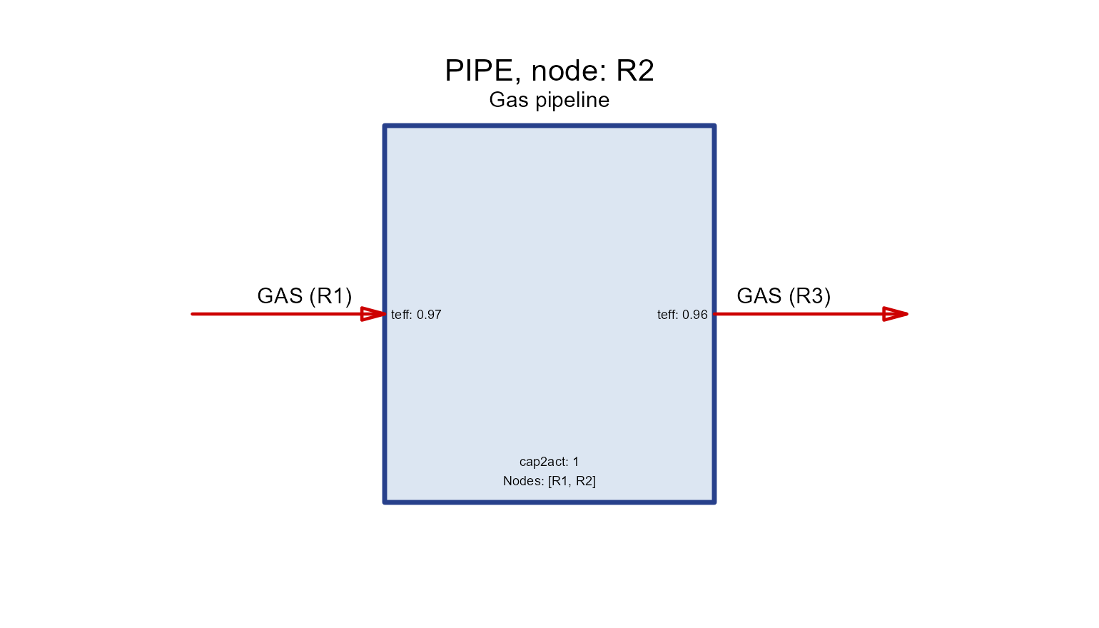

storage

Shifts a commodity across time. seff holds the charging/discharging/holding efficiencies (inpeff/outeff/stgeff) and cap2stg is the storage duration.

STG_ELC <- newStorage(
  name = "STG_ELC", desc = "Battery", commodity = "ELC",
  seff = data.frame(inpeff = 0.9, outeff = 0.9, stgeff = 0.999),
  cap2stg = 4,                                   # 4 hours of storage per unit power
  aux  = data.frame(acomm = "LITHIUM", unit = "kt"),
  aeff = data.frame(acomm = "LITHIUM", ncap2ainp = 0.25))  # material per new capacity
draw(STG_ELC)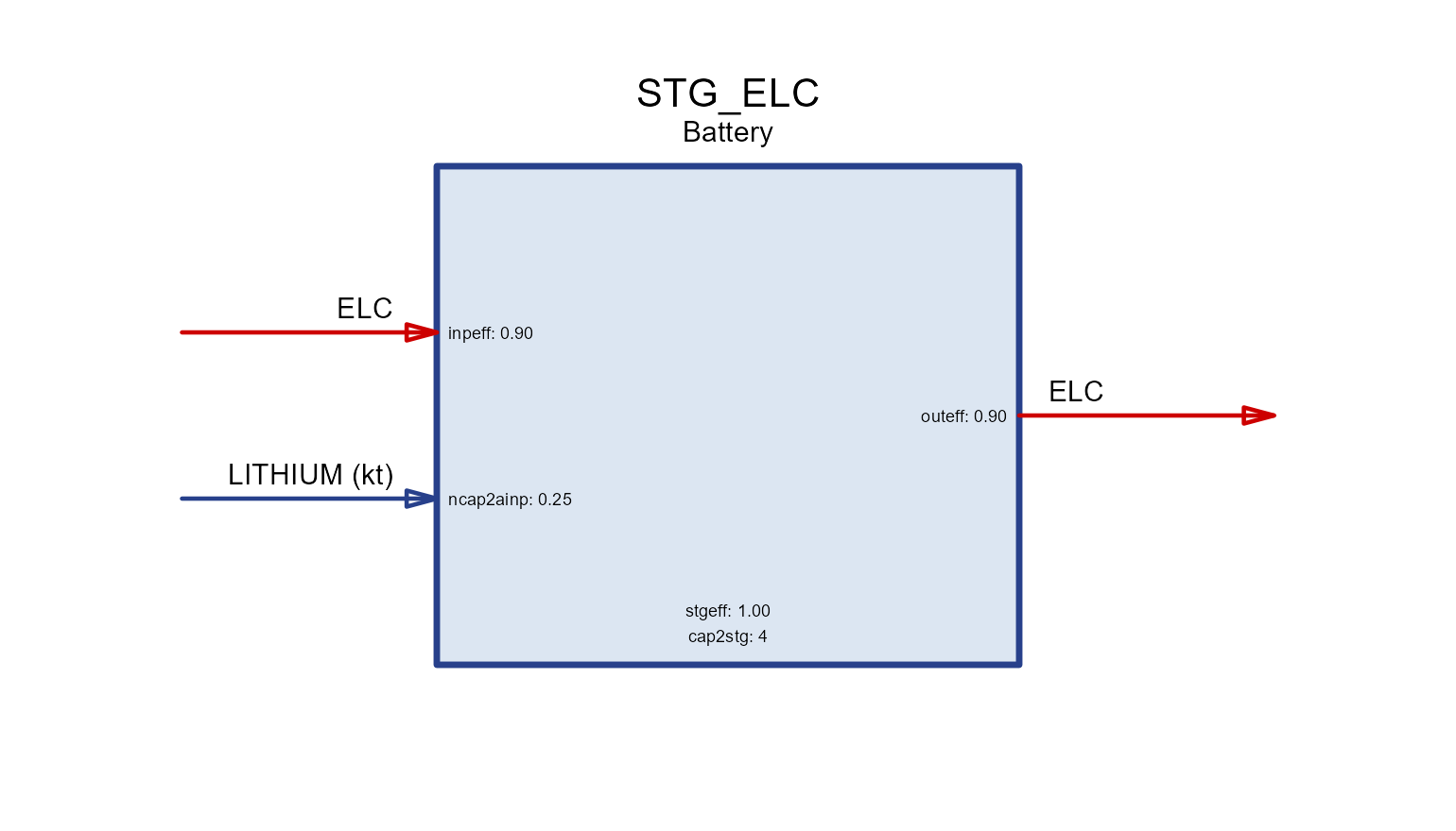

Anatomy of a technology

A technology converts input commodities into output commodities. Read its diagram left-to-right through four internal stages:

   input(s)  ──▶  use  ──▶  activity  ──▶  output(s)
             cinp2use   use2cact      cact2cout

cinp2use — how much of a common use each unit of a commodity input provides (e.g. converting fuels to a common energy basis).
use2cact — use to the technology’s activity (the central variable that all costs, availability and capacity are tied to).
cact2cout — activity to each output commodity (efficiency / yield). All three default to 1.

BOILER <- newTechnology(
  name = "BOILER", desc = "Gas boiler",
  input  = data.frame(comm = "GAS",  unit = "PJ"),
  output = data.frame(comm = "HEAT", unit = "PJ"),
  ceff = data.frame(comm = c("GAS", "HEAT"),
                    cinp2use  = c(1,  NA),
                    cact2cout = c(NA, 0.9)),   # 90% efficiency
  cap2act = 1)
draw(BOILER)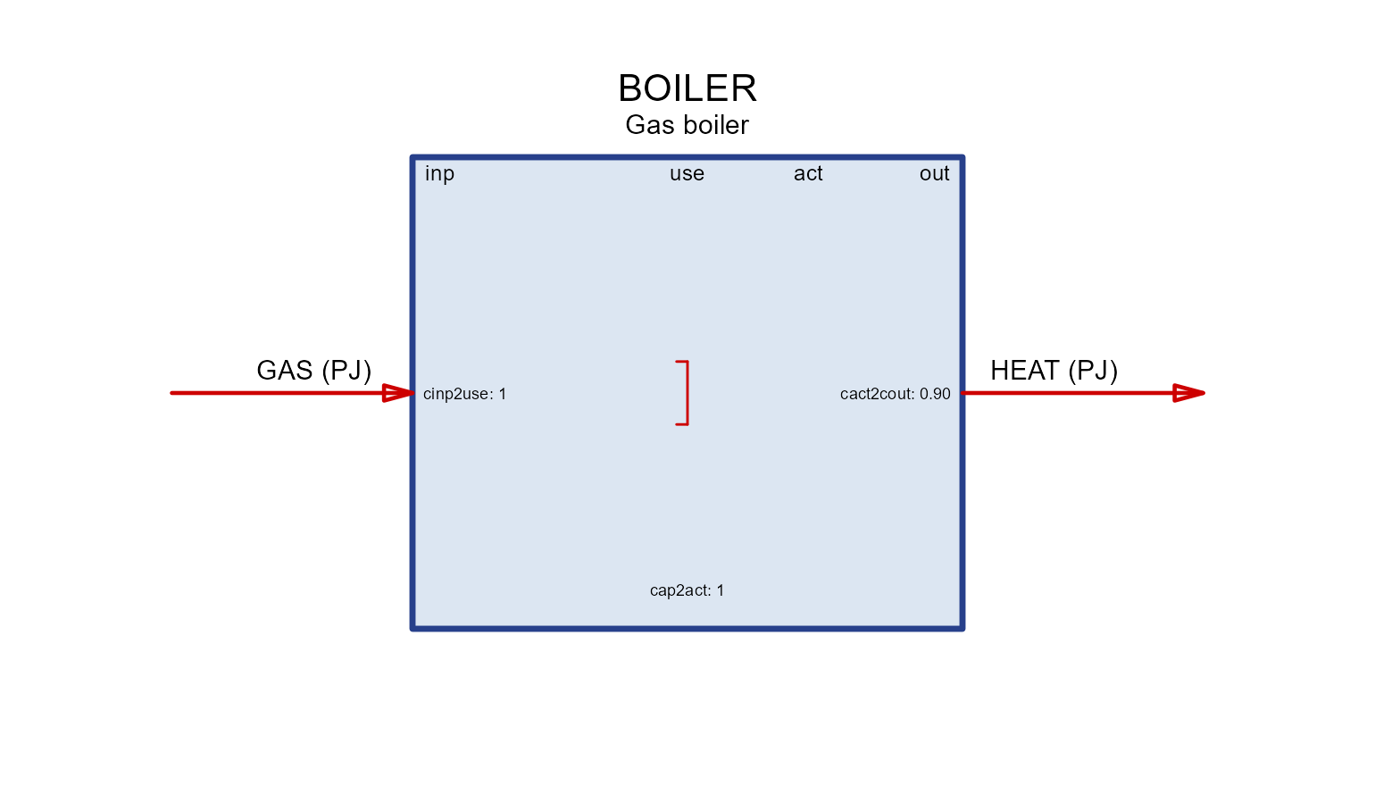

The four column headers in the box (inp, use, act, out) are exactly these stages; each coefficient is printed next to the flow it scales.

Groups and shares

When several commodities are interchangeable on the input (or output) side, put them in a group. A group is converted to use once (via ginp2use in geff), and each member’s contribution is bounded by a share (share.lo/share.up/share.fx). cinp2ginp converts each commodity into the group’s common unit.

CHP <- newTechnology(
  name = "CHP", desc = "Co-firing plant (coal + biomass)",
  input = data.frame(comm = c("COA", "BIO"), group = "fuel", unit = "PJ"),
  output = data.frame(comm = "ELC", unit = "GWh"),
  group = data.frame(group = "fuel", desc = "Blended fuel", unit = "PJ"),
  geff  = data.frame(group = "fuel", ginp2use = 1),
  ceff  = data.frame(comm = c("COA", "BIO", "ELC"),
                    cinp2ginp = c(1, 1, NA),
                    cact2cout = c(NA, NA, 0.4),
                    share.up  = c(1.0, 0.3, NA)),   # at most 30% biomass
  cap2act = 8.76)
draw(CHP)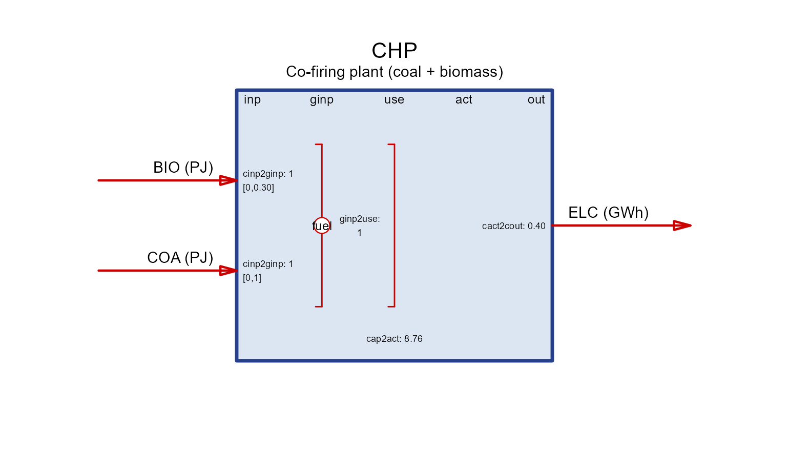

The share range is drawn in square brackets next to each grouped commodity.

Activity, capacity and units

Everything a technology does is measured by its activity. Installed capacity limits the maximum activity through the scalar cap2act:

cap2act — “how much product (activity, or output commodity if identical) is produced per unit of capacity”. For a power plant with capacity in GW, cap2act = 8.76 gives a maximum activity of 8.76 GWh per GW per year (8760 h, scaled to the cost/energy units in use).
Capacity itself is bounded in the capacity slot: stock (pre-existing), cap.lo/up/fx (total), ncap.lo/up/fx (new builds) and ret.lo/up/fx (retirement). Availability factors af/afs bound activity within capacity.

Capacity in input vs. output units

Because capacity is tied to activity, whether it is expressed in input or output units depends on where you place the efficiency. Keep cinp2use = 1 and put the loss on the output (cact2cout = 0.9) and activity tracks the input — so capacity is in fuel-input units. Move the efficiency to the input side instead and capacity becomes an output rating:

# capacity rated on OUTPUT (e.g. a 1 GW_e turbine): activity == output
BOILER_out <- newTechnology(
  name = "BOILER_out", desc = "Boiler rated by heat output",
  input  = data.frame(comm = "GAS",  unit = "PJ"),
  output = data.frame(comm = "HEAT", unit = "PJ"),
  ceff = data.frame(comm = c("GAS", "HEAT"),
                    cinp2use  = c(1 / 0.9, NA),   # efficiency on the input side
                    cact2cout = c(NA, 1)),        # activity == heat output
  cap2act = 1)
draw(BOILER_out)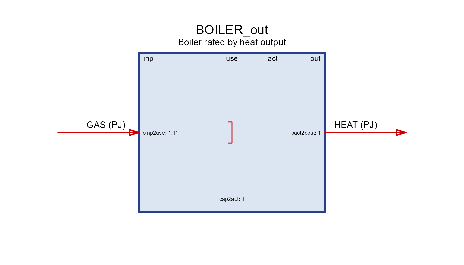

Both boilers have the same 90% efficiency; they differ only in what a unit of capacity means (fuel input vs. heat output).

Auxiliary commodities

Auxiliary commodities are extra flows tracked alongside the main conversion — emissions, land, water, critical materials, by-products. They are declared in aux and linked in aeff by a coefficient named <driver>2a<out|inp>:

the driver is what scales the flow: cinp (commodity input), cout (output), act (activity), cap (installed capacity), ncap (new capacity), or storage terms;
…2aout produces the aux commodity (emissions, land, by-products); …2ainp consumes it (materials, energy).

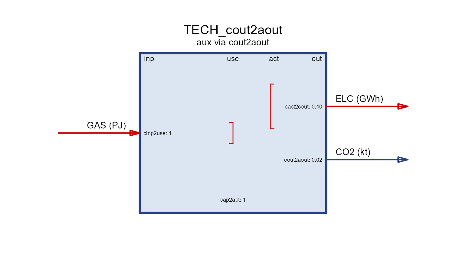
Each tab isolates one driver on the same base technology (GAS → ELC).

aux_tech <- function(param, value, acomm = "AUX", unit = "unit") {
  aeff <- data.frame(acomm = acomm, stringsAsFactors = FALSE)
  aeff[[param]] <- value
  newTechnology(
    name = paste0("TECH_", param), desc = paste0("aux via ", param),
    input  = data.frame(comm = "GAS", unit = "PJ"),
    output = data.frame(comm = "ELC", unit = "GWh"),
    ceff   = data.frame(comm = c("GAS", "ELC"), cinp2use = c(1, NA), cact2cout = c(NA, 0.4)),
    aux    = data.frame(acomm = acomm, unit = unit),
    aeff   = aeff)
}

act2aout

Produced per unit of activity — the usual way to attach combustion CO2.

draw(aux_tech("act2aout", 56, "CO2", "kt"))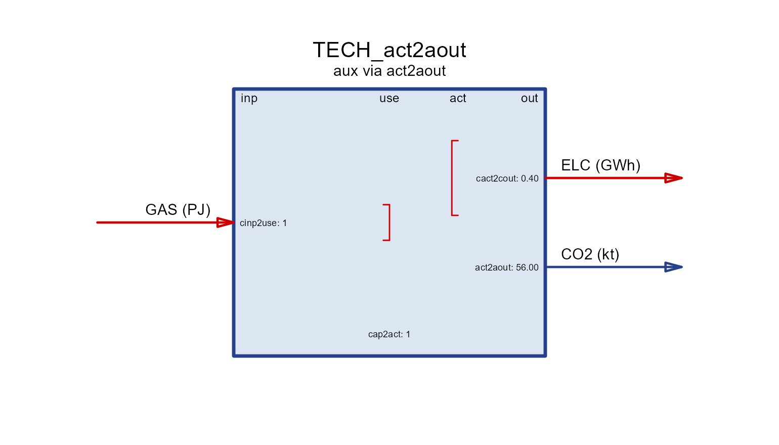

cout2aout

Produced per unit of output commodity.

draw(aux_tech("cout2aout", 0.02, "CO2", "kt"))

cinp2aout

Produced per unit of input commodity (e.g. process emissions from a feedstock).

draw(aux_tech("cinp2aout", 0.05, "CO2", "kt"))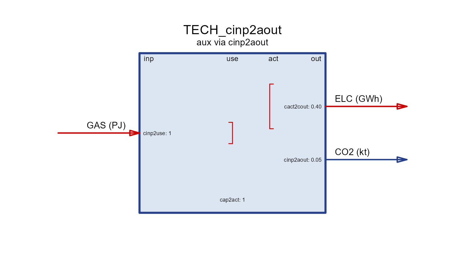

cap2aout

Produced per unit of installed capacity (e.g. land occupied while the plant stands).

draw(aux_tech("cap2aout", 10, "LAND", "km2"))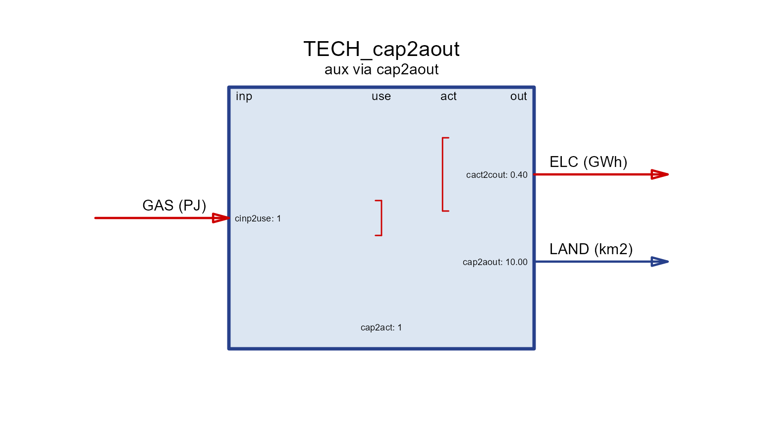

ncap2aout

Produced per unit of new capacity (one-off, e.g. construction emissions).

draw(aux_tech("ncap2aout", 3, "CO2", "kt"))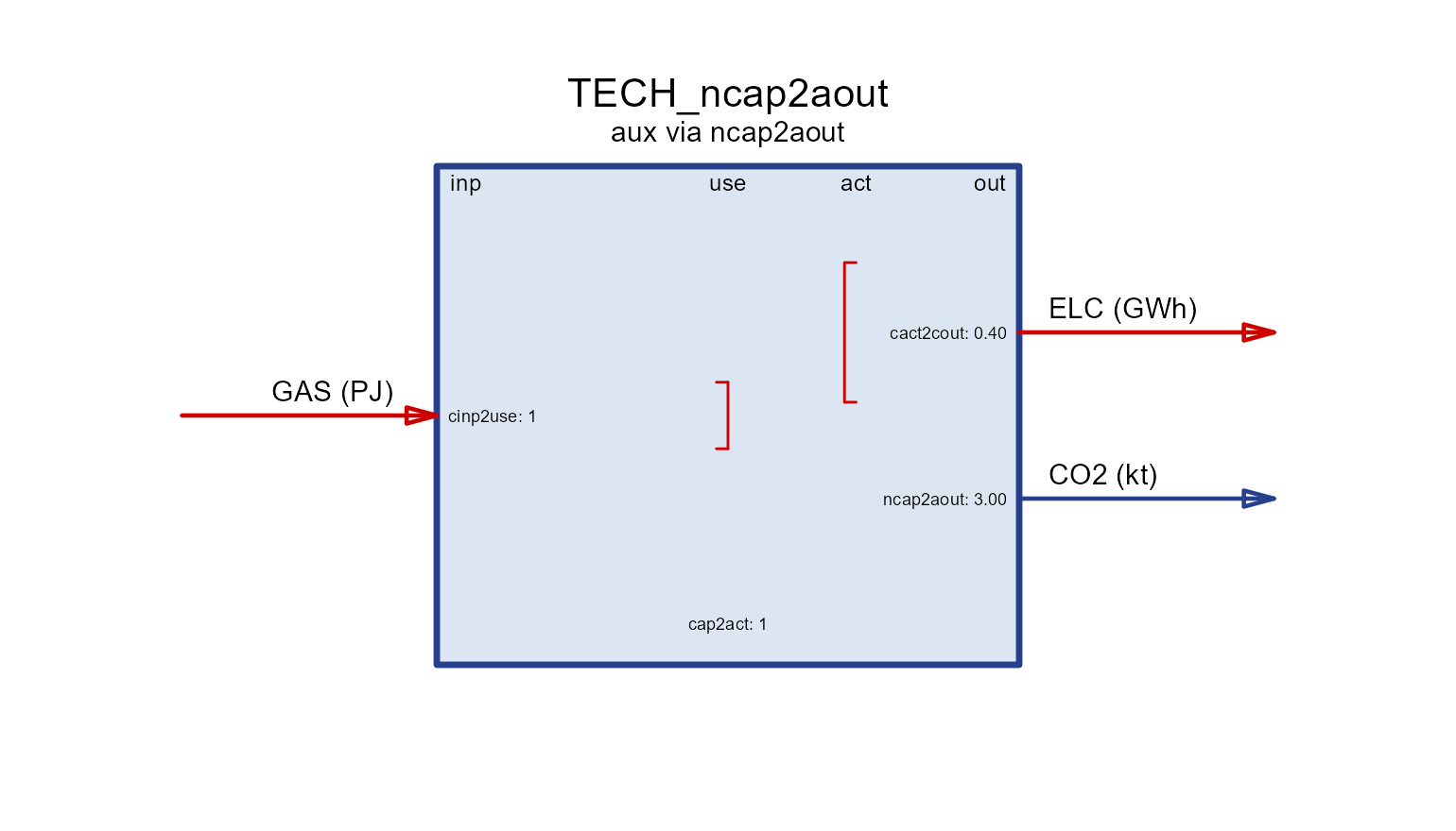

act2ainp

Consumed per unit of activity (e.g. water or electricity used to run).

draw(aux_tech("act2ainp", 0.1, "WATER", "Mm3"))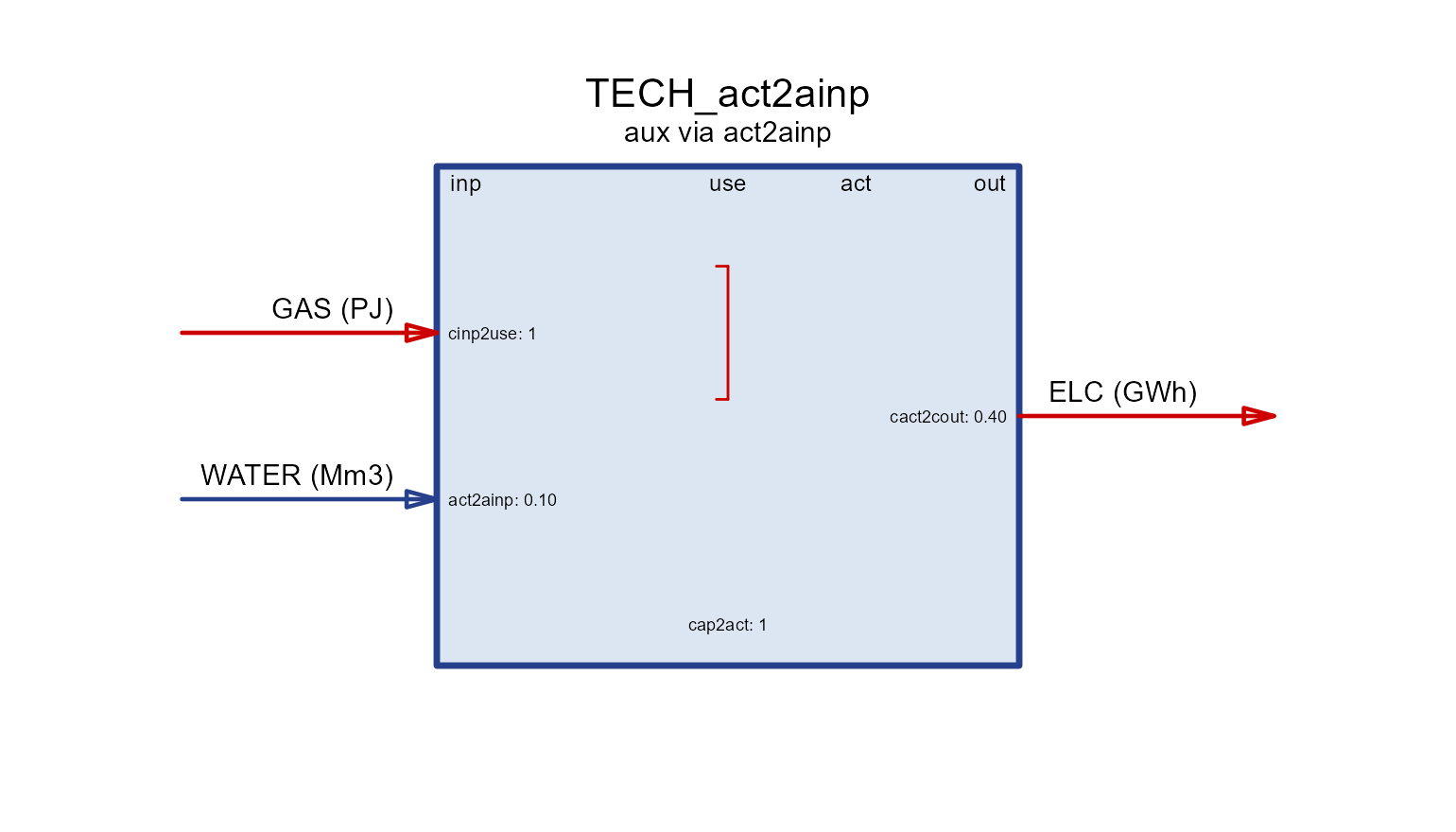

cap2ainp

Consumed per unit of capacity — a stock of material tied up in the plant.

draw(aux_tech("cap2ainp", 4, "STEEL", "kt"))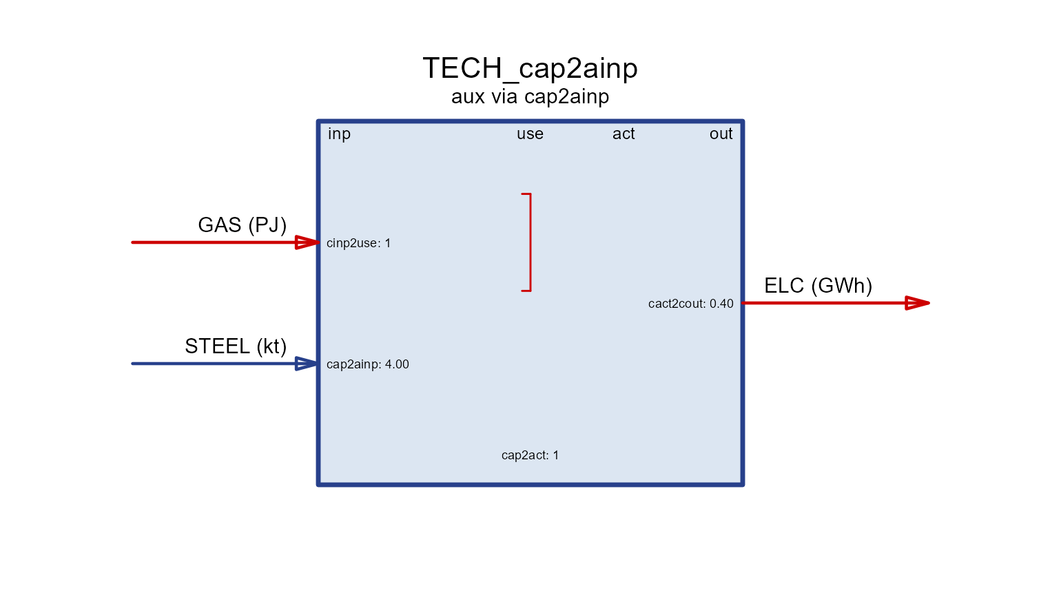

ncap2ainp

Consumed per unit of new capacity — materials used to build (e.g. lithium per GWh of battery, as in the storage example above).

draw(aux_tech("ncap2ainp", 0.25, "LITHIUM", "kt"))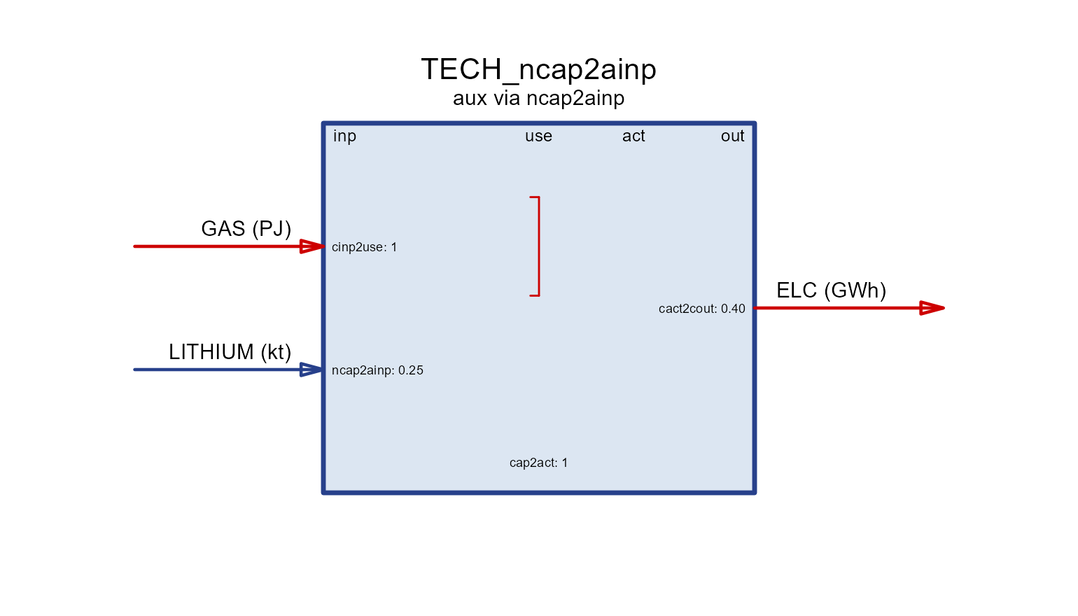

Timeframe (operating frequency)

A technology operates at a timeframe — the level of the calendar it is dispatched on. By default it is the finest (highest-frequency) timeframe among the commodities it uses: a plant producing hourly ELC runs hourly, while one producing only annual STEEL runs annually. Set timeframe = to force a coarser level (e.g. run an electricity plant at "SEASON" rather than "HOUR" to shrink the model).

newTechnology(
  name = "WIND", input = data.frame(comm = character()),
  output = data.frame(comm = "ELC", unit = "GWh"),
  timeframe = "HOUR")            # dispatch hourly (else inferred from commodities)