Time resolution: calendars and slices
Source:vignettes/articles/time-resolution.Rmd
time-resolution.RmdWhy sub-annual time matters
Annual averages hide what makes energy systems hard: the sun sets, wind stalls, demand peaks in the evening. A model that balances electricity once a year sees none of it — storage is pointless, solar looks dispatchable, peak capacity is free. A calendar gives the model sub-annual time slices, and the slice count is the main dial between realism and model size:
| calendar | structure | slices |
|---|---|---|
utopia_annual |
one annual slice | 1 |
utopia_seasons |
4 seasons × day/night/peak | 12 |
utopia_s4h24 |
4 seasons × 24 hours | 96 |
utopia_m12h24 |
12 months × 24 hours | 288 |
d365 |
365 days | 365 |
Model variables scale roughly linearly with slices — the 96-slice UTOPIA base case solves in seconds on GLPK, the 288-slice variant is noticeably heavier.
The make_timetable() grammar
A calendar’s structure is a nested named list: each
element is a level (e.g. SEASON,
HOUR), holding its slices. Slice names must be
alphanumeric (they become set elements in the solver files). The
simplest form lists slice names — the year is divided equally:
tt <- make_timetable(list(
  SEASON = c("WIN", "SPR", "SUM", "AUT"),
  HOUR   = paste0("h", formatC(0:23, width = 2, flag = "0"))
))
head(tt)          # 4 x 24 = 96 leaf slices, equal shares
#>    ANNUAL SEASON   HOUR   slice      share weight
#>    <char> <char> <char>  <char>      <num>  <num>
#> 1: ANNUAL    AUT    h00 AUT_h00 0.01041667      1
#> 2: ANNUAL    AUT    h01 AUT_h01 0.01041667      1
#> 3: ANNUAL    AUT    h02 AUT_h02 0.01041667      1
#> 4: ANNUAL    AUT    h03 AUT_h03 0.01041667      1
#> 5: ANNUAL    AUT    h04 AUT_h04 0.01041667      1
#> 6: ANNUAL    AUT    h05 AUT_h05 0.01041667      1
Unequal shares are given per slice; a nested
list(<share>, <LEVEL> = ...) attaches child
levels. UTOPIA’s 12-slice calendar makes peak hours short and winter
nights long:
tt12 <- make_timetable(list(
  SEASON = list(
    WIN = list(1 / 4, HOUR = list(DAY =  9 / 24, NGT = 12 / 24, PK = 3 / 24)),
    SPR = list(1 / 4, HOUR = list(DAY = 11 / 24, NGT = 11 / 24, PK = 2 / 24)),
    SUM = list(1 / 4, HOUR = list(DAY = 12 / 24, NGT =  9 / 24, PK = 3 / 24)),
    AUT = list(1 / 4, HOUR = list(DAY = 11 / 24, NGT = 11 / 24, PK = 2 / 24))
  )
))
head(tt12)
#>    ANNUAL SEASON   HOUR   slice      share weight
#>    <char> <char> <char>  <char>      <num>  <num>
#> 1: ANNUAL    AUT    DAY AUT_DAY 0.11458333      1
#> 2: ANNUAL    AUT    NGT AUT_NGT 0.11458333      1
#> 3: ANNUAL    AUT     PK  AUT_PK 0.02083333      1
#> 4: ANNUAL    SPR    DAY SPR_DAY 0.11458333      1
#> 5: ANNUAL    SPR    NGT SPR_NGT 0.11458333      1
#> 6: ANNUAL    SPR     PK  SPR_PK 0.02083333      1
From timetable to calendar
newCalendar() turns a timetable into a
calendar object. Note that name is the
first argument — always pass the timetable by name
(timetable =), or name name/desc
so the timetable lands in the right slot:
cal <- newCalendar(timetable = tt, name = "s4h24")
cal@name
#> [1] "s4h24"
nrow(cal@slice_share)          # slices with their share of the year
#> [1] 101
head(as.data.frame(cal@slice_share), 3)
#>    slice share weight
#> 1 ANNUAL  1.00      1
#> 2    AUT  0.25      1
#> 3    SPR  0.25      1
cal@timeframe_rank             # levels, coarsest (ANNUAL) to finest
#> ANNUAL SEASON   HOUR
#>      1      2      3
The derived slots do the bookkeeping the model needs:
-
@slice_share— each slice’s share of the year (the weight used whenever slice values are aggregated); -
@timeframes— the slice sets at every level (ANNUAL,SEASON, …); -
@timeframe_rank— the level hierarchy; a commodity’stimeframepicks the level it is balanced on.
autoplot() draws the nested structure:
autoplot(cal)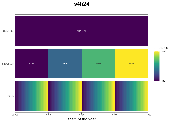
Ready-made calendars
The package ships a calendars list, built by
data-raw/calendars.R with exactly the grammar above —
including the whole UTOPIA family:
names(calendars)
#> [1] "season_dn"                      "d365"
#> [3] "utopia_annual"                  "utopia_seasons"
#> [5] "utopia_s4h24"                   "utopia_m12h24"
#> [7] "d365_h24"                       "d365_h24_subset_1day_per_month"
calendars$utopia_seasons@desc
#> [1] "UTOPIA: 4 seasons x 3 dayparts (DAY/NIGHT/PEAK), 12 slices"
Pick one and pass it to newModel(calendar = ...); the
UTOPIA vignettes use calendars$utopia_s4h24 throughout.
Slice-string helpers
Slice names encode time; a few helpers translate between encodings:
hour2HOUR(c(0, 13, 23))        # hour of day -> "h00" "h13" "h23"
#> [1] "h00" "h13" "h23"
yday2YDAY(c(1, 365))           # day of year -> "d001" "d365"
#> [1] "d001" "d365"
head(tsl_formats)              # known slice-name formats (a dataset)
#> [1] "d364"     "d365"     "d366"     "d364_h24" "d365_h24" "d366_h24"
tsl2dtm() / dtm2tsl() convert slice strings
to/from date-times — useful when joining model output with observed
hourly data.
Timeframes: commodities and processes
Every commodity carries a timeframe — the calendar level
it is balanced on. Fuels are typically
ANNUAL; electricity HOUR:
ELC <- newCommodity("ELC", timeframe = "HOUR")    # balanced every slice
COA <- newCommodity("COA", timeframe = "ANNUAL")  # balanced once a year
A process operates at the finest timeframe among its
commodities (a gas plant producing hourly ELC is dispatched
hourly), overridable via newTechnology(timeframe = ...) —
see the model bricks article for
details. The practical consequence: raising the calendar’s resolution
refines only the commodities and processes whose timeframes
follow it — annual bookkeeping stays cheap.
Choosing a resolution
- Start coarse (
utopia_seasons-like, ~12 slices) while the model structure is in flux — solves are instant. - Move to hour-within-season (
utopia_s4h24, 96) once storage, VRE profiles or peak pricing matter — intra-day dynamics need real hours. - Full-year hourly detail (
utopia_m12h24, 288 ord365+hours) is for final runs; check tractability withmodel_size()first.
The UTOPIA vignettes build one model and run it on these calendars interchangeably — resolution is a configuration choice, not a rewrite.