
Key functions
- Query and plot:
getData(),autoplot(),gg_heatmap(). - Compare:
compare_scenarios(),compare_models(),compare_inputs(). - Publish:
levcost(),report(),report_templates().
energyRt renders reports — self-contained
HTML/PDF/Word datasheets — for technologies and storages, whole models
and repositories, solved scenarios, and scenario comparisons. Reports
and the levelized costs (levcost()) that
feed them are derived artifacts: both are cached on disk and
re-computed only when their inputs change. This article tours the layer
— what renders where, how the caching works, and how to compare
scenarios.
Read the solution, then ask a question
A solved scenario stores decoded variables in
modOut. If several solver runs exist, make the run choice
explicit before querying:
scenario_runs(scen)
scen <- read_solution(scen, run = "julia-highs")
getData() is the common query interface for model
declarations, interpolated parameters, and solution variables. Name the
variable first, then filter on its dimensions:
cap <- getData(scen, "vTechCap", year = 2030, merge = TRUE)
gen <- getData(scen, "vTechAct", comm = "ELC", merge = TRUE)
ems <- getData(scen, "vEmsFuelTot", comm = "CO2", merge = TRUE)
merge = TRUE joins useful labels and mappings into the
returned table. Leave it off when you need only the native variable
keys. Keep the query in code and save a derived table only when it is a
deliverable; modOut remains the source of truth.
Plot while you explore
autoplot() methods cover model objects, dimensions,
comparisons, and several result objects. They return ggplot
objects, so normal layers and themes work:
autoplot(calendars$s4_hp3, fill = "share", border = "grey50") +
  labs(title = "Four seasons with day, night, and peak slices") +
  theme_minimal()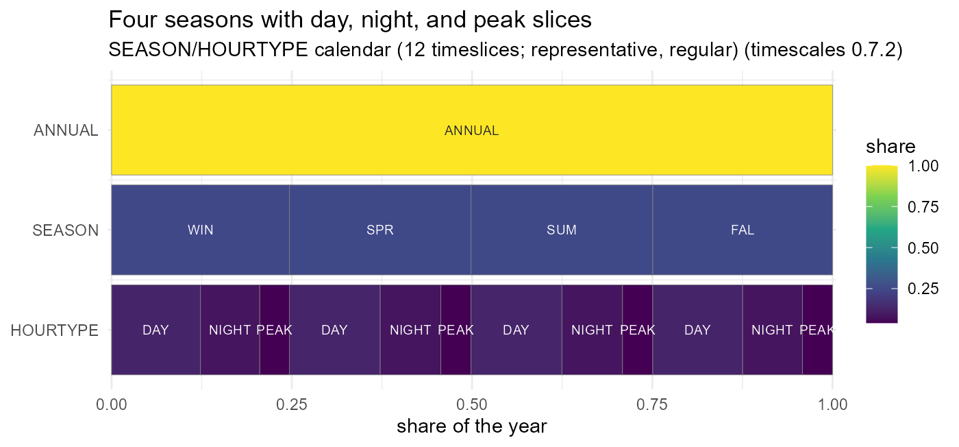
Choose the view that matches the data rather than forcing everything
into one chart. gg_heatmap() suits values indexed by two
calendar dimensions; autoplot(weather, calendar = ...)
offers heatmap, line, and area styles; autoplot(supply) and
related methods show declared points and interpolated paths. For solved
scenarios, query a focused table with getData() and build a
custom ggplot when the reporting question is specific.
Compare while exploring
For an ad-hoc variable comparison, pass several scenario names or
objects to getData(). This is the fastest way to check one
hypothesis before building a structured comparison or report.
Everything lands under a throwaway project here;
open_project() anchors the registry, the object stores, and
the two derived-artifact folders (reports/,
levcosts/) in one call:
proj <- file.path(tempdir(), "rep-demo")
dir.create(proj, showWarnings = FALSE)
open_project(proj)
#> energyRt project: C:/Users/admin/AppData/Local/Temp/RtmpmmGelk/rep-demo (0 registered scenarios)
A technology to price and report on:
PP <- newTechnology(
  "PP", desc = "Gas power plant",
  input  = list(comm = "GAS", unit = "GWh"),
  output = list(comm = "ELC", unit = "GWh"),
  ceff   = data.frame(comm = "GAS", cinp2use = 0.55),
  invcost = data.frame(invcost = 800),
  fixom = data.frame(fixom = 20), varom = data.frame(varom = 2),
  af = data.frame(af.up = 0.85),
  vintage = data.frame(olife = 25L), cap2act = 8.76)
Levelized costs, cached
levcost() prices a technology (LCOE), storage (LCOS), or
trade route (LCOT). method = "auto" uses a closed-form
engine when the process qualifies and falls back to a small solver run
otherwise:
lc <- levcost(PP, fuel_costs = c(GAS = 25), discount = 0.06,
              base_year = 2025, verbose = FALSE)
round(as.numeric(lc$levcost_npv), 2)
#> [1] 58.55
The result was also written to the on-disk cache, keyed by the technology’s content hash plus the assumptions. Re-pricing the identical question returns instantly from disk:
lc2 <- levcost(PP, fuel_costs = c(GAS = 25), discount = 0.06,
               base_year = 2025)
#> levcost: cached result is current: C:/Users/admin/AppData/Local/Temp/RtmpmmGelk/rep-demo/levcosts/PP@8099a340.rds (force = TRUE to recompute)
list.files(get_levcost_cache_path())
#> [1] "PP@8099a340.rds" "PP@8099a340.yml"
Anything that changes the answer — the technology’s data,
discount, fuel prices, the method — is part of the cache
key, so a stale hit is impossible; force = TRUE recomputes
regardless, and cache = FALSE skips the cache entirely. For
objects saved in a store the cache moves into the owning folder
(<scenario>/levcost/, a model store entry’s
levcost/); the project-level levcosts/ above
is the tier for in-memory objects.
Rendering a datasheet
report() renders a technology datasheet — parameters,
the draw() diagram, and (with levcost =) the
levelized-cost section. The same rule places the output: saved objects
render inside their own folder’s reports/, in-memory
objects into the project-level reports/ tier:
f <- report(PP, levcost = lc, format = "html", open = FALSE)
#> Report written to C:\Users\admin\AppData\Local\Temp\RtmpmmGelk\rep-demo\reports\report_PP.html
basename(f)
#> [1] "report_PP.html"
A report is skip-if-current: the rendered file
carries a sidecar (*.report.yml) keying the object content,
the template content, the arguments, and the levcost identity. Repeating
the call re-renders nothing:
f <- report(PP, levcost = lc, format = "html", open = FALSE)
#> Report up to date: C:\Users\admin\AppData\Local\Temp\RtmpmmGelk\rep-demo\reports\report_PP.html (force = TRUE to re-render)
Editing the technology, the template, or any argument invalidates the
key; force = TRUE re-renders unconditionally. Formats:
format = takes any of "html",
"pdf", "tex", "docx" (PDF needs a
LaTeX toolchain).
Model and scenario reports
Container reports split by role: report(model) documents
the assumptions (configuration, inventories,
per-process sheets), while report(scenario) documents the
results of a solved scenario — status,
generation/capacity charts, costs, emissions; run = renders
any recorded run, and template = "full" switches to the
comprehensive page-broken layout with maps and branding. Reporting a
single process from a container injects its container-priced levelized
cost:
report(scen)                       # results overview -> <scenario>/reports/
report(scen, run = "julia_highs")  # another recorded run
report(scen, template = "full")    # comprehensive, page-broken layout
report(scen, name = "PP")          # one process, priced in this scenario
The process sections follow your groups: a named list of
process names or regular expressions, passed as groups = or
stored once in mod@misc$report_groups (a scenario inherits
its model’s). Without groups the report shows a representative sample of
up to 12 processes; groups = "topology" groups
automatically by structure. levcost = TRUE adds a
levelized-cost comparison — an overall chart, one chart per group, and
the ranked table — ex-ante on a model, ex-post on a solved scenario; a
process datasheet requested from a container also compares the process
with its structural peers:
mod@misc$report_groups <- list(Coal = "_coal_", Wind = c("^R._win", "WOFF"))
report(mod)                        # one section per group + "Ungrouped"
report(mod, groups = FALSE)        # ignore the stored groups: sample of 12
report(mod, levcost = TRUE)        # ex-ante LCOE comparison, per group
report(scen, levcost = TRUE)       # ex-post, from the solved scenario
report(mod, name = "PP")           # datasheet + "vs peers" chart
Figures in reports carry captions rather than in-plot titles, and
faceted charts cap at 16 panels with their height following the layout.
Custom templates get the same behaviour from
report_fig(p, width, caption = ).
The shipped templates are listed by report_templates();
custom .Rmd templates build on the exported
report_* helper family and are passed via
template = "<path>".
Element datasheets
Every model component has a report() method —
commodities, supply, demand, trade, import/export, weather, taxes and
subsidies, user constraints, calendars, horizons, configurations, and
user costs each render a one-object datasheet from their own shipped
template. A supply datasheet charts availability and cost by region
(autoplot(sup, style = "bar") /
style = "regions" draw the same views directly; an
unlimited availability shows as a translucent full-height bar):
report(COA)                          # a commodity datasheet
report(SUP_COA)                      # a supply datasheet
report(mod, name = "SUP_COA")        # the same, found inside a model
report(mod, name = "X", class = "demand")   # narrow a name lookup
An object can carry its own default template in
misc$report (also the techspec report: key) —
a template name or a file path; an explicit template =
argument always wins:
SUP_COA@misc$report <- "my_supply_sheet.Rmd"
report(SUP_COA)                      # renders my_supply_sheet.Rmd
Comparing scenarios
compare_scenarios() takes a named list of solved
scenarios (or one scenario plus runs = to compare its
recorded runs) and returns a classed comparison — overview, per-variable
deltas against the base, and the largest movers; autoplot()
charts it and report() renders the comparative report:
cmp <- compare_scenarios(list(BASE = base, CO2CAP = capped))
cmp                                # printed overview + top deltas
autoplot(cmp)                      # faceted comparison charts
report(cmp, open = FALSE)          # the comparative report (report_scenarios)
compare_models() diffs two models’ declarations
(inventory by content hash, config, then per-slot drill-down), and
compare_inputs() diffs two interpolated scenarios’
parameter stores — the tool for “same model, different numbers?”
questions. For quick ad-hoc comparisons, plain getData()
across scenarios remains the one-liner (see Solving models):
Where everything lands
<project>/
├── reports/              # reports of in-memory objects (temporary tier)
├── levcosts/             # levcost cache of in-memory objects
├── scenarios/<scen>/
│   ├── reports/          # this scenario's reports
│   └── levcost/          # its levcost cache
└── models/<name>/
    ├── reports/          # a stored model's reports
    └── levcost/          # its levcost cache
Both tiers are caches of derived artifacts: safe to delete at any time, rebuilt on demand, and never consulted for anything but skipping work.