Storage

library(energyRt)
library(ggplot2)

What a storage is

Every other process in energyRt turns a flow into another flow now. A storage is the only one that moves energy between timeslices: it holds a level, and the level carries across the calendar.

That gives it three separate physical things, which for a long time energyRt squeezed into one:

	what it is	unit	slot
charger	how fast it can fill	power	`@input`
reservoir	how much it can hold	energy	`@storage`
discharger	how fast it can empty	power	`@output`

A battery is an inverter plus a stack of cells. A pumped-hydro plant is a pump, a reservoir and a turbine. An electric car is a charge point, a battery and a motor. In each case the three are sized — and priced — separately, and the interesting modelling questions are about the ratios between them.

Declare the commodity first, with its unit, then the process:

ELC <- newCommodity(
  name      = "ELC",
  desc      = "Electricity",
  unit      = "MWh",
  timeframe = "HOUR"
)

STG_BTR <- newStorage(
  name      = "STG_BTR",
  desc      = "Lithium-ion battery (6-hour)",
  commodity = "ELC",
  output    = list(
    comm    = "ELC",
    unit    = "MWh",
    invcost = 12144                       # EUR/MW  -- the inverter
  ),
  storage   = list(
    comm    = "ELC",
    unit    = "MWh",
    invcost = 8081                        # EUR/MWh -- the cells
  ),
  duration  = 6,                          # a 6-hour battery
  vintage   = data.frame(olife = 15L)
)
draw(STG_BTR)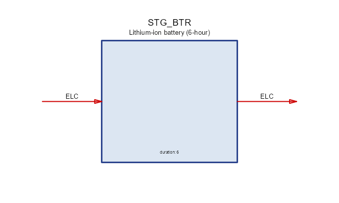

commodity = "ELC" is shorthand: it fills all three roles at once. There is no @commodity slot — the argument is folded into @input, @storage and @output when the object is built, so a storage never carries two answers to “what does it consume”. Naming a role explicitly, as @output and @storage are named above, overrides the shorthand for that role only.

unit is descriptive: it is the unit of the commodity on that side, carried for reporting and convert(), and never reaches the solver. Capacity units are not declared — they follow from cap2act, which is why the storing side has none.

The three commodities need not be the same

This is the part that changes what you can model. @storage$comm is what the store holds; @input$comm and @output$comm are what it exchanges. When all three coincide you have a battery. When they do not:

H2 <- newCommodity(
  name      = "H2",
  desc      = "Hydrogen",
  unit      = "MWh",
  timeframe = "HOUR"
)

STG_H2 <- newStorage(
  name      = "STG_H2",
  desc      = "Salt-cavern hydrogen store with electrolyser and fuel cell",
  commodity = "H2",                       # what it HOLDS
  input     = list(
    comm    = "ELC",                      # electrolyser
    unit    = "MWh",
    invcost = 226174
  ),
  output    = list(
    comm    = "ELC",                      # fuel cell
    unit    = "MWh"
  ),
  storage   = list(
    comm    = "H2",                       # the cavern
    unit    = "MWh",
    invcost = 112
  ),
  seff      = data.frame(
    inpeff  = 0.70,
    outeff  = 0.50
  ),
  vintage   = data.frame(olife = 25L)
)
draw(STG_H2)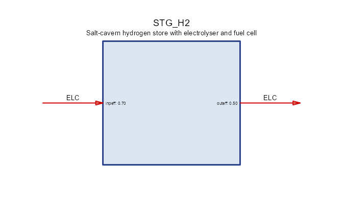

@seff$inpeff and $outeff are cross-commodity conversion factors here — input→stored and stored→output — the same role cinp2use plays for a technology. When the three commodities coincide they are the round-trip efficiencies they have always been, and nothing changes.

Before this, the same system needed an electrolyser, a store, a fuel cell, and an artificial H2 commodity whose only job was to join them. On a two-day test model the fused object reproduces the decomposition’s objective exactly (193.142857 on GLPK, Julia/HiGHS, Pyomo and GAMS alike) in 149 variables and 151 constraints instead of 251 and 257.

The saving is structural rather than clever: the artificial commodity’s balance rows disappear along with the two technologies.

An electric car is the case where this really bites. ELC is shared with the grid, so a composed model needs an artificial on-board commodity to stop the motor drawing from the mains while driving. Disjoint availability profiles do not save you — the profile sits on the technology, not on the commodity.

The whole object at a glance

Everything a storage can carry, and where the rest of this article covers it.

slot	what it holds	section
`@name`, `@desc`	identity	above
`@input`, `@output`, `@storage`	the three parts: commodity, unit, capacity, cost	above, and Sizing the parts
`@duration`, `@inp2out`	ratios tying the parts together	Sizing the parts
`@fullYear`	where the cycle closes	`@fullYear`
`@startLevel`	endowment at the start of a cycle	`@startLevel`
`@seff`	storing / charging / discharging efficiency	The three commodities, Losses
`@af`	availability of the level and of the two flows	Availability
`@capacity`	whole-object stock, bounds and retirement	Capacity, stock and retirement
`@invcost`, `@fixom`, `@varom`	economics	Costs
`@aux`, `@aeff`	auxiliary commodities	Auxiliary commodities
`@weather`	weather-driven availability	Weather
`@region`	where it may be built	Regions and variants
`@cluster`, `@vintage`	variants of one object	Regions and variants
`@optimizeRetirement`	let the model retire early	Capacity, stock and retirement
`@misc`	anything else, untouched	—

`@fullYear`: where the cycle closes

The single most consequential flag on a storage, and the easiest to get wrong.

fullYear = TRUE (the default) — one cycle over the whole year. Energy put in during April can come out in October.
fullYear = FALSE — one cycle per parent timeframe. On a day/hour calendar every day is an independent loop and nothing crosses midnight.

Cheap generation is unavailable on the February day, and all demand falls there, so the store is the only cheap way to serve it — and only if energy may cross the boundary between the two days.

# A bundled calendar: one representative day per month, 24 hours each. Its
# timeslices are DATED (`d015_h00`), which the reporting tools below need.
cal <- calendars$d365_h24_subset_1day_per_month
slices <- unique(cal@timetable$timeslice)
jan <- grep("^d015_", slices, value = TRUE)     # the January day
feb <- grep("^d046_", slices, value = TRUE)     # the February day

COA <- newCommodity(
  name      = "COA",
  desc      = "Steam coal",
  unit      = "MWh",
  timeframe = "ANNUAL"
)

SUP_COA <- newSupply(
  name      = "SUP_COA",
  desc      = "Coal supply",
  commodity = "COA",
  supply    = data.frame(cost = 1)
)

ECOA <- newTechnology(
  name    = "ECOA",
  desc    = "Cheap coal plant, unavailable on the February day",
  input   = list(comm = "COA", unit = "MWh"),
  output  = list(comm = "ELC", unit = "MWh"),
  invcost = data.frame(invcost = 10),
  af      = data.frame(timeslice = feb, af.up = 0),   # off in February
  vintage = data.frame(olife = 30L),
  cap2act = 1
)

EPEAK <- newTechnology(
  name    = "EPEAK",
  desc    = "Expensive peaking plant, always available",
  input   = list(comm = "COA", unit = "MWh"),
  output  = list(comm = "ELC", unit = "MWh"),
  invcost = data.frame(invcost = 5000),
  vintage = data.frame(olife = 30L),
  cap2act = 1
)

STG_YEAR <- newStorage(
  name      = "STG_YEAR",
  desc      = "Electricity store, one cycle over the whole year",
  commodity = "ELC",
  invcost   = list(invcost = 1),
  vintage   = data.frame(olife = 30L),
  fullYear  = TRUE
)

STG_DAY <- newStorage(
  name      = "STG_DAY",
  desc      = "The same store, but cycling once per day",
  commodity = "ELC",
  invcost   = list(invcost = 1),
  vintage   = data.frame(olife = 30L),
  fullYear  = FALSE
)

DEM_ELC <- newDemand(
  name      = "DEM_ELC",
  desc      = "Electricity demand, February day only",
  commodity = "ELC",
  demand    = data.frame(timeslice = feb, demand = 10)
)

The two stores are identical apart from @fullYear, so each gets its own repository and model:

repo_year <- newRepository(
  name = "repo_year",
  COA, ELC, SUP_COA, ECOA, EPEAK, STG_YEAR, DEM_ELC
)

repo_day <- newRepository(
  name = "repo_day",
  COA, ELC, SUP_COA, ECOA, EPEAK, STG_DAY, DEM_ELC
)

mod_year <- newModel(
  name     = "fy_year",
  desc     = "Storage cycling over the year",
  region   = "R1",
  horizon  = newHorizon(2020),
  discount = 0,
  calendar = cal,
  repo     = repo_year
)

mod_day <- newModel(
  name     = "fy_day",
  desc     = "Storage cycling every day",
  region   = "R1",
  horizon  = newHorizon(2020),
  discount = 0,
  calendar = cal,
  repo     = repo_day
)

scen_year <- solve_model(mod_year, name = "fy_year")
#> Solver directory:  scenarios/fy-year_d365-h24-subset-1day-per-month/script/glpk 
#> Writing files: 0.3s
#> Starting  GLPK 
#> 0.15s
#> Reading solution: 0.1s
scen_day <- solve_model(mod_day, name = "fy_day")
#> Solver directory:  scenarios/fy-day_d365-h24-subset-1day-per-month/script/glpk 
#> Writing files: 0.3s
#> Starting  GLPK 
#> 0.12s
#> Reading solution: 0.08s

getData(scen_year, "vObjective", merge = TRUE)$value
#> [1] 9962.545
getData(scen_day, "vObjective", merge = TRUE)$value
#> [1] 14607300

With the cycle closed inside each day the store cannot help at all and the model falls back on the expensive plant. The flag is not a detail.

@fullYear was inert before energyRt v0.80 — every storage cycled within its parent timeframe whatever the flag said, which made multi-day and seasonal storage silently unrepresentable. It surfaced when a converted PyPSA-Eur battery came out 2.1x oversized and idle 6,624 hours of 8,760.

`@startLevel`: an endowment, once per cycle

@startLevel says how much is in the store at the start of a cycle. It has no timeslice column on purpose: the slice is derived from where the cycle closes, not chosen. It is an annual quantity, so a store cycling daily receives its share, not the whole thing 365 times over.

STG_HYD <- newStorage(
  name       = "STG_HYD",
  desc       = "Reservoir hydro with an inherited initial filling",
  commodity  = "ELC",
  startLevel = data.frame(
    region     = "R1",
    year       = 2020L,
    startLevel = 500
  ),
  vintage    = data.frame(olife = 60L)
)
STG_HYD@startLevel
#>   vintage cluster region year startLevel
#> 1    <NA>    <NA>     R1 2020        500

Sizing the parts

@duration and @inp2out are the two ratios that tie the three parts together. Both are bounds, on (storage, region, year):

duration = reservoir / discharger   [hours]
inp2out  = charger   / discharger   [dimensionless]

duration = 6 fixes the ratio — a 6-hour battery. A range lets the model choose:

STG_FLEX <- newStorage(
  name      = "STG_FLEX",
  desc      = "Battery whose energy-to-power ratio the model chooses",
  commodity = "ELC",
  output    = list(comm = "ELC", unit = "MWh", invcost = 12),
  storage   = list(comm = "ELC", unit = "MWh", invcost = 8),
  duration  = data.frame(
    duration.lo = 2,
    duration.up = 8
  ),
  vintage   = data.frame(olife = 15L)
)
STG_FLEX@duration
#>   vintage cluster region year duration duration.lo duration.up duration.fx
#> 1    <NA>    <NA>   <NA>   NA       NA           2           8          NA

A one-sided range opens the other side: duration.up = 8 means “up to 8 hours” and does not quietly inherit a lower bound of 1.

An optimised ratio only means something when the reservoir is priced — with energy free the model simply takes the longest duration allowed. Given a cost on both sides, and both sides binding, it lands strictly inside the range.

@inp2out works the same way for the charger. Leave it out and the charger is sized with the discharger; give it a range and asymmetric hardware — a fast charger with a slow fuel cell, or a pump smaller than its turbine — becomes a decision rather than an assumption.

Structure follows data

A part carrying only a commodity name gets no capacity variable at all. Naming a commodity is metadata, not data; only a stock, a bound or a price materialises vStorageInpCap / vStorageStgCap. Everywhere else the ratio is inlined onto vStorageOutCap, which is exactly the older, smaller model.

That is why adding all of this moved nothing: a storage written the old way keeps one capacity variable and its previous LP, to the row.

variable	side	unit
`vStorageInpCap`	charger	power
`vStorageStgCap`	reservoir	energy
`vStorageOutCap`	discharger	power

vStorageCap no longer exists. It meant power, and vStorageStgCap means energy — one syllable apart. Rather than leave a name whose meaning had to be guessed, it was renamed vStorageOutCap, so the old name resolves to nothing instead of returning the wrong quantity. Use getData(scen, "vStorageOutCap").

Rates and energy: `cap2act`

A charger is a rate — 7 kW is 7 kW whether you model the year in hours or in four-hour blocks. A reservoir is an amount — 60 kWh is 60 kWh either way. energyRt keeps flows as quantities within a timeslice, so the rate has to be converted at the bound:

vStorageInp[.,s] <= cinp.up * cap2act * vStorageInpCap * pTimesliceShare[s]

cap2act is capacity → annual flow, exactly as on a technology. It defaults to 8760, the hours in a year, which makes a capacity read as commodity per hour on any calendar:

calendar	share per slice	`8760 × share`
8760 × 1 h	1/8760	1
2190 × 4 h	4/8760	4
365 × 1 d	1/365	24
1 × annual	1	8760

Write cap.fx = 7 and you get 7 per hour in every row of that table. If your commodity is TWh against GW capacity rather than GWh, use 8.76.

A calendar is a YEAR, so say which part of it you mean

cap2act only reads as “per hour” if a timeslice really is an hour, and that is a property of the calendar, not of the storage. Declare 24 timeslices as a whole year and each is 365 hours long, so cap.fx = 7 quietly means 0.019 per hour.

The fix is not to adjust cap2act — that just renames the confusion. It is to say the calendar covers one day out of the year:

YF  <- 1 / 365
cal <- newCalendar(
  timetable     = make_timetable(
    struct        = list(ANNUAL = "ANNUAL", HOUR = hrs),
    year_fraction = YF
  ),
  year_fraction = YF,
  name          = "one_day"
)

Each slice then has share = 1/8760 — a real hour — and the timeslice weight comes out as 365, so costs annualise as “this day, repeated all year”. The bundled representative-day calendars work the same way, which is why their leaf share is 1/8760 rather than 1/288.

Before this, the bound carried no share factor, so a capacity meant “commodity per timeslice”. The same cap.fx = 7 allowed 7 per hour on a 24 × 1-hour calendar and 1.75 per hour on a 6 × 4-hour one — refine the resolution and every store silently became weaker. vStorageStgCap is deliberately not scaled: energy is energy.

This is also what makes duration honest. With the discharger a per-hour rate and the reservoir an amount, duration = vStorageStgCap / vStorageOutCap is an hour count — so duration = 6 on a 10 MW discharger gives exactly 60 MWh.

PyPSA does the same thing from the other end

PyPSA’s state-of-charge equation is

soc[t] = (1-standing_loss)^eh · soc[t-1] + eff_store·eh·p_store − eh·p_dispatch/eff_dispatch

where eh is elapsed hours. Its p_* variables are rates, so no limit constraint is scaled at all — neither p ≤ p_nom nor soc ≤ e_nom. energyRt puts the conversion on the bound instead of in the variable; the physics is identical. Note energyRt already agreed on the decay term, which has always been (pStorageStgEff)^(pTimesliceShare) — the same compounding by elapsed time.

What aggregation still costs you

Making the rating resolution-independent does not make a coarse calendar adequate. Discharge in a slice is bounded by three things:

(1) out <= cout.up · cap2act · outCap · share[s]
(2) out / outeff <= level[s]
(3) level[s] <= af.up · stgCap

For a 6 h / 10 MW battery (60 MWh), only (1) changes with resolution:

calendar	flow bound (1)	energy bound (2)+(3)	binds
hourly	10 MWh	60 MWh	flow
daily	240 MWh	60 MWh	energy
day/night	43,800 MWh	60 MWh	energy

So on coarse slices the power rating goes slack and the store is governed by its energy capacity alone. Hence:

The power rating binds only when the timeslice is shorter than the storage’s discharge duration.

Worse, the cycle count collapses. N timeslices allow at most ⌊N/2⌋ cycles, so on a day/night calendar a 6-hour battery can perform exactly one cycle a year — 60 MWh moved, against roughly 21,900 MWh for a store that really cycles daily. On a single annual timeslice there is no dynamic at all: the cyclic balance pairs the slice with itself and collapses to inpeff·inp = out/outeff.

A store whose cycle is shorter than one timeslice is therefore understated, not approximated. Representing ~365 daily cycles needs on the order of 730 timeslices — sub-6-hourly resolution. That is a property of temporal aggregation, not something the units fix can recover.

Losses: `@seff`

@seff carries all three efficiencies, and they are applied at different places in the level equation:

column	applies to	meaning
`inpeff`	charging	fraction of the input that reaches the level
`outeff`	discharging	level drawn per unit delivered is `1/outeff`
`stgeff`	holding	retention per hour, compounded as `stgeff^share`

stgeff is the one to watch: it is a rate, raised to the timeslice share, so 0.999 is a per-hour retention and not a per-timeslice one. That is what keeps a self-discharge assumption stable when the calendar is refined.

STG_BTR_LOSS <- newStorage(
  name      = "STG_BTR_LOSS",
  desc      = "Battery with round-trip and self-discharge losses",
  commodity = "ELC",
  duration  = 6,
  seff      = data.frame(
    inpeff = 0.95,
    outeff = 0.95,
    stgeff = 0.999
  ),
  vintage   = data.frame(olife = 15L)
)
STG_BTR_LOSS@seff
#>   vintage cluster region year timeslice stgeff inpeff outeff
#> 1    <NA>    <NA>   <NA>   NA      <NA>  0.999   0.95   0.95

Efficiencies may vary by region, year and timeslice, so a store that ages or a cavern that leaks more in summer is a matter of extra rows.

Availability: `@af`

@af bounds the level and the two flows as fractions of their capacities. Three families share the slot:

columns	bounds
`af.lo` / `af.up` / `af.fx`	the level, against `vStorageStgCap`
`cinp.lo` / `cinp.up` / `cinp.fx`	charging, against the charger
`cout.lo` / `cout.up` / `cout.fx`	discharging, against the discharger

Each accepts region, year and timeslice, so the bound can follow the calendar. A reservoir kept above a minimum head, and a grid connection that may not charge during the evening peak:

STG_RES <- newStorage(
  name      = "STG_RES",
  desc      = "Reservoir with a minimum head and a charging curfew",
  commodity = "ELC",
  storage   = list(comm = "ELC", unit = "MWh", invcost = 40),
  af        = data.frame(
    timeslice = c(NA, "d046_h18"),
    af.lo     = c(0.15, NA),              # never draw below 15% full
    cinp.up   = c(NA, 0)                  # no charging in that slice
  ),
  vintage   = data.frame(olife = 40L)
)
STG_RES@af
#>   vintage cluster region year timeslice af.lo af.up af.fx cinp.up cinp.fx
#> 1    <NA>    <NA>   <NA>   NA      <NA>  0.15    NA    NA      NA      NA
#> 2    <NA>    <NA>   <NA>   NA  d046_h18    NA    NA    NA       0      NA
#>   cinp.lo cout.up cout.fx cout.lo
#> 1      NA      NA      NA      NA
#> 2      NA      NA      NA      NA

NA in a key column means “every member of it”, so the first row applies in every timeslice and the second only in the named one. .fx overrides the matching .lo/.up pair.

Capacity, stock and retirement

@capacity describes the object as a whole, in the same shape a technology uses: existing stock, bounds on total capacity (cap.*), bounds on new builds (ncap.*), and bounds on retirement (ret.*). Per-part capacity lives on @input / @output / @storage; @capacity is the place for what is true of the storage itself.

STG_FLEET <- newStorage(
  name      = "STG_FLEET",
  desc      = "Existing battery fleet with a build limit",
  commodity = "ELC",
  capacity  = data.frame(
    region  = "R1",
    year    = 2020L,
    stock   = 120,                        # already built
    ncap.up = 50                          # at most 50 more in this year
  ),
  vintage   = data.frame(olife = 15L)
)
STG_FLEET@capacity
#>   vintage cluster region year stock cap.lo cap.up cap.fx ncap.lo ncap.up
#> 1    <NA>    <NA>     R1 2020   120     NA     NA     NA      NA      50
#>   ncap.fx ret.lo ret.up ret.fx
#> 1      NA     NA     NA     NA

@optimizeRetirement = TRUE lets the model retire capacity before its operational life ends — worth it when a store is cheap to build and expensive to keep. It only takes effect when the model or scenario also enables it, so the flag on the object is a permission rather than an instruction.

Costs: `@invcost`, `@fixom`, `@varom`

Three slots, on the three things you can spend money on:

slot	charged on	key columns
`@invcost`	new capacity	`invcost`, `wacc`, `payback`, `eac`, `retcost`
`@fixom`	installed capacity, per year	`fixom`
`@varom`	flows and level, per timeslice	`inpcost`, `outcost`, `stgcost`

@invcost and @fixom on the object price the whole store; the same names inside @input / @output / @storage price one part, which is what the battery at the top of this article does. @varom splits by what is charged: inpcost per unit charged, outcost per unit discharged, stgcost per unit held.

STG_PRICED <- newStorage(
  name      = "STG_PRICED",
  desc      = "Battery priced on capacity and on every unit moved",
  commodity = "ELC",
  duration  = 6,
  invcost   = data.frame(invcost = 8081), # EUR/MWh on new capacity
  fixom     = data.frame(fixom = 5),      # EUR/MW/yr on the whole store
  varom     = data.frame(
    inpcost = 0.5,
    outcost = 0.5
  ),
  vintage   = data.frame(olife = 15L)
)
STG_PRICED@varom
#>   vintage cluster region year timeslice inpcost outcost stgcost
#> 1    <NA>    <NA>   <NA>   NA      <NA>     0.5     0.5      NA

wacc, payback and eac behave exactly as on a technology: see the technology article rather than a second copy here.

Auxiliary commodities: `@aux` and `@aeff`

An auxiliary commodity is anything the store consumes or produces that is not one of its three roles — lithium for the cells, water for a reservoir, land. @aux declares the commodity and its unit; @aeff says what it is proportional to.

The @aeff column names read source2target, so ncap2ainp is auxiliary input per unit of new capacity, and cout2aout is auxiliary output per unit discharged:

column	auxiliary flow driven by
`ncap2ainp` / `ncap2aout`	new capacity (a build-time material)
`cap2ainp` / `cap2aout`	installed capacity (something held)
`cinp2ainp` / `cinp2aout`	charging
`cout2ainp` / `cout2aout`	discharging
`stg2ainp` / `stg2aout`	the level itself
`ncap2stg`	new capacity, on the storing side

MAT <- newCommodity(
  name = "MAT",
  desc = "Battery-grade lithium",
  unit = "kt"
)

STG_MAT <- newStorage(
  name      = "STG_MAT",
  desc      = "Battery that consumes lithium when it is built",
  commodity = "ELC",
  duration  = 6,
  aux       = data.frame(
    acomm = "MAT",
    unit  = "kt"
  ),
  aeff      = data.frame(
    acomm     = "MAT",
    ncap2ainp = 0.25                      # kt of lithium per MW built
  ),
  vintage   = data.frame(olife = 15L)
)
STG_MAT@aeff[, c("acomm", "ncap2ainp")]
#>   acomm ncap2ainp
#> 1   MAT      0.25

Weather

@weather multiplies availability by a named weather object, so an inflow series or an ambient-temperature derating drives the bounds. The coefficients mirror @af: waf.* scales the level bound, wcinp.* charging and wcout.* discharging.

STG_HYD_W <- newStorage(
  name      = "STG_HYD_W",
  desc      = "Reservoir hydro driven by an inflow series",
  commodity = "ELC",
  weather   = data.frame(
    weather  = "WHYD",                    # a newWeather() object in the repo
    wcinp.fx = 1                          # inflow drives charging
  ),
  vintage   = data.frame(olife = 60L)
)

The weather object itself must be in the same repository. Availability, not capacity, is what weather scales — a dry year does not shrink the reservoir.

Several weather factors may act on the same bound — they multiply, on every backend. Verified across GLPK and Julia/HiGHS on a two-factor process, which agree on the objective to ten digits.

Regions and variants

@region restricts where the storage may be built — leave it empty and it is available everywhere in the model.

@cluster and @vintage turn one object into several. A vintage is a build period with its own lifetime and costs; a cluster is a parallel variant, such as a resource grade. Both are declared once and then referenced from the vintage / cluster column that nearly every other slot carries, which is how a 2020 battery and a 2050 battery can differ in cost without becoming two objects.

STG_VINT <- newStorage(
  name      = "STG_VINT",
  desc      = "Battery with two build vintages",
  commodity = "ELC",
  region    = "R1",
  vintage   = data.frame(
    vintage = c("v2020", "v2050"),
    start   = c(2020L, 2050L),
    end     = c(2049L, 2100L),
    olife   = c(12L, 20L)
  ),
  storage   = list(
    comm    = c("ELC", "ELC"),
    unit    = c("MWh", "MWh"),
    vintage = c("v2020", "v2050"),
    invcost = c(8081, 3200)               # cells get cheaper
  )
)
STG_VINT@vintage
#>   vintage region cluster start  end olife
#> 1   v2020   <NA>    <NA>  2020 2049    12
#> 2   v2050   <NA>    <NA>  2050 2100    20
STG_VINT@storage[, c("comm", "vintage", "invcost")]
#>   comm vintage invcost
#> 1  ELC   v2020    8081
#> 2  ELC   v2050    3200

Every slot that carries a vintage (or cluster) column can be split this way, so the two vintages differ only where you say they do. See the variants material for how the two interact.

Reading the result: `storage_duration()`

A level series tells you how full the store is. It does not tell you the thing that decides what technology you need: how much of that energy is cycling within a few hours, and how much is sitting there for weeks.

storage_duration() splits the level into duration bands by nested floors. For a window of w hours, the floor is the energy that never leaves the store across some w-hour stretch — energy committed for at least that long. Floors are nested, so successive differences partition the level with no overlap and no remainder: the bands sum back to vStorageLevel exactly.

A solar-plus-battery system on the same bundled calendar gives it something to decompose: generation only in the middle of the day, demand in the evening.

hr <- as.integer(sub(".*_h", "", slices))

SOL <- newCommodity(
  name      = "SOL",
  desc      = "Solar irradiation",
  unit      = "MWh",
  timeframe = "HOUR"
)

SUP_SOL <- newSupply(
  name      = "SUP_SOL",
  desc      = "Solar resource, daylight hours only",
  commodity = "SOL",
  supply    = data.frame(
    timeslice = slices,
    cost      = 0,
    ava.up    = ifelse(hr >= 8 & hr <= 16, 100, 0)
  )
)

ESOL <- newTechnology(
  name    = "ESOL",
  desc    = "Solar PV",
  input   = list(comm = "SOL", unit = "MWh"),
  output  = list(comm = "ELC", unit = "MWh"),
  invcost = data.frame(invcost = 10),
  vintage = data.frame(olife = 30L),
  cap2act = 8760
)

DEM_EVE <- newDemand(
  name      = "DEM_EVE",
  desc      = "Evening-peaked electricity demand",
  commodity = "ELC",
  demand    = data.frame(
    timeslice = slices,
    demand    = ifelse(hr >= 17 & hr <= 22, 10, 1)
  )
)

STG_BTR_SOL <- newStorage(
  name      = "STG_BTR_SOL",
  desc      = "Battery paired with the solar plant",
  commodity = "ELC",
  invcost   = list(invcost = 1),
  vintage   = data.frame(olife = 30L),
  fullYear  = TRUE
)

repo_sol <- newRepository(
  name = "repo_sol",
  SOL, ELC, SUP_SOL, ESOL, EPEAK, STG_BTR_SOL, DEM_EVE
)

sol_mod <- newModel(
  name     = "solar_battery",
  desc     = "Solar plus a battery on one day per month",
  region   = "R1",
  horizon  = newHorizon(2020),
  discount = 0,
  calendar = cal,
  repo     = repo_sol
)

scen <- solve_model(sol_mod, name = "solar_battery")
#> Solver directory:  scenarios/solar-battery_d365-h24-subset-1day-per-month/script/glpk 
#> Writing files: 0.2s
#> Starting  GLPK 
#> 0.25s
#> Reading solution: 0.08s

d <- storage_duration(scen)                 # 12h / 1d / 1w / 30d by default

# One panel per representative day: this calendar's days are a month apart, so
# plotting them on one continuous axis would draw lines across gaps that are not
# in the model.
d$day <- format(d$datetime, "%b")
d$hour <- as.integer(format(d$datetime, "%H"))
ggplot(d, aes(hour, value, fill = duration)) +
  geom_area() +
  facet_wrap(~factor(day, levels = unique(d$day))) +
  scale_fill_viridis_d(direction = -1, name = "Duration") +
  labs(x = "Hour of the representative day", y = "Storage level") +
  theme_bw()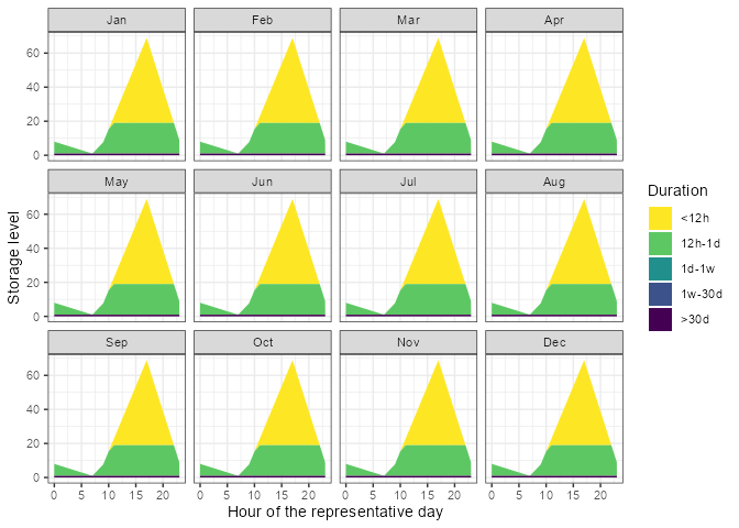

Every band here is short: a day-per-month calendar has no way to represent energy held from spring to autumn, so the long bands can only show as a flat floor. A genuinely seasonal split needs a contiguous full-year calendar.

A full year, on measured wind and solar

vre_cf is a year of hourly capacity factors for one wind and one solar resource, derived from the MERRA-2 reanalysis. Its slice column is already in the d365_h24 vocabulary, so it drops onto the bundled hourly calendar:

str(vre_cf)
#> 'data.frame':    8760 obs. of  3 variables:
#>  $ slice: chr  "d001_h00" "d001_h01" "d001_h02" "d001_h03" ...
#>  $ solar: num  0 0 0 0 0 0 0 0 0.002 0.013 ...
#>  $ wind : num  0.995 0.966 0.89 0.84 0.81 ...
colMeans(vre_cf[, c("solar", "wind")])
#>     solar      wind 
#> 0.1256643 0.2488839

The model is deliberately spare: two weather-driven plants, a gas backstop, a cheap store and a constant demand. With demand flat, everything the store does is forced by the resource rather than by the load.

cal <- calendars$d365_h24

# The capacity factor belongs on the TECHNOLOGY, as an hourly availability
# bound. Putting it on a supply's `ava.up` instead caps the resource in
# absolute terms, so the plant can never be built larger than one unit however
# cheap it is, and the backstop quietly covers the rest.
ESOL <- newTechnology(
  name    = "ESOL",
  desc    = "Solar PV",
  output  = list(comm = "ELC", unit = "MWh"),
  af      = data.frame(timeslice = vre_cf$slice, af.up = vre_cf$solar),
  invcost = data.frame(invcost = 700),
  vintage = data.frame(olife = 25L),
  cap2act = 8760
)

EWIN <- newTechnology(
  name    = "EWIN",
  desc    = "Wind turbine",
  output  = list(comm = "ELC", unit = "MWh"),
  af      = data.frame(timeslice = vre_cf$slice, af.up = vre_cf$wind),
  invcost = data.frame(invcost = 1300),
  vintage = data.frame(olife = 25L),
  cap2act = 8760
)

# Cheap, and its ENERGY far cheaper than its power, so the model would rather
# keep a surplus than spill it. Price the store highly and the optimum is
# simply to curtail: the level never carries, and every band above a day comes
# out empty.
STG_BTR_VRE <- newStorage(
  name      = "STG_BTR_VRE",
  desc      = "Cheap store, energy and power sized separately",
  commodity = "ELC",
  output    = list(comm = "ELC", unit = "MWh", invcost = 20),  # power, per MW
  storage   = list(comm = "ELC", unit = "MWh", invcost = 1),   # energy, per MWh
  seff      = data.frame(inpeff = 0.95, outeff = 0.95),
  vintage   = data.frame(olife = 15L),
  fullYear  = TRUE
)

DEM_VRE <- newDemand(
  name      = "DEM_VRE",
  desc      = "Constant electricity demand",
  commodity = "ELC",
  demand    = data.frame(timeslice = vre_cf$slice, demand = 1)
)

# ... plus the ELC and GAS commodities, SUP_GAS and the EPEAK backstop;
# the whole script is data-raw/vre_storage_duration.R

scen_vre <- solve_model(mod_vre, solver = solver_options$julia_highs)
vre_storage_duration <- storage_duration(scen_vre)

The answer is a system with no gas built at all: 2.4 units of solar and 3.0 of wind generate 9064 against a demand of 8760, the 3.5% gap being the store’s round-trip loss rather than spilled energy. To do that it buys a 520 MWh store — three weeks of demand — and runs it as a season-length reservoir.

Solve that one on julia/HiGHS, not GLPK — at 8760 timeslices the difference is minutes, which is why the result is precomputed and shipped as vre_storage_duration rather than solved while this page builds.

ggplot(vre_storage_duration, aes(datetime, value, fill = duration)) +
  geom_area() +
  scale_fill_viridis_d(direction = -1, name = "Duration") +
  labs(x = NULL, y = "Storage level") +
  theme_bw()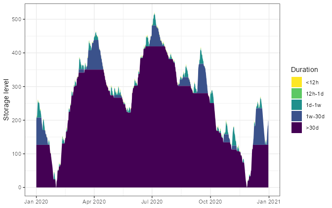

Now the split is worth reading. The store is not one thing doing one job: a thin band cycles within the day, while most of the energy is committed for more than thirty days — charged when wind and sun are abundant and released a season later.

tapply(vre_storage_duration$value, vre_storage_duration$duration, sum)
#>        <12h      12h-1d       1d-1w      1w-30d        >30d 
#>    3848.461    6035.640   56860.498  173581.134 2141880.391

Those long bands are exactly what a coarse calendar cannot see. Reading them off a model with @fullYear = FALSE, or with timeslices longer than the cycle you care about, would return near-zero — not because the storage is short-duration, but because the model was never able to say otherwise.

Change the bands with width (in hours) and name them with labels. A store that cycles within its parent timeframe cannot hold energy longer than that cycle, so its long bands come out near zero — a property of the model, not a failure of the split.

Despite its name in the original IDEEA script, this is not a moving average. An average would blur the bands into each other and would not sum back to the level.